Hand drawn sketch | Models made in CC4 with ZBrush | Textures in Substance Painter | Paint over in Photoshop | Renders, Animation, VFX with AI. Each 5-8 hours spread over a couple days.
As I continue to explore the use of AI tools to enhance my 3D character creation process, I discover they can be incredibly useful during the previsualization phase to see what a character might ultimately look like in production. I selectively use AI to enhance and accelerate my creative process, not to replace it or use it as an end to end solution.
This paper presents an introduction to the color pipelines behind modern feature-film visual-effects and animation.
Authored by Jeremy Selan, and reviewed by the members of the VES Technology Committee including Rob Bredow, Dan Candela, Nick Cannon, Paul Debevec, Ray Feeney, Andy Hendrickson, Gautham Krishnamurti, Sam Richards, Jordan Soles, and Sebastian Sylwan.
In video terms gamut is normally related to as the full range of colours and brightness that can be either captured or displayed.
Generally speaking all color gamuts recommendations are trying to define a reasonable level of color representation based on available technology and hardware. REC-601 represents the old TVs. REC-709 is currently the most distributed solution. P3 is mainly available in movie theaters and is now being adopted in some of the best new 4K HDR TVs. Rec2020 (a wider space than P3 that improves on visibke color representation) and ACES (the full coverage of visible color) are other common standards which see major hardware development these days.
To compare and visualize different solution (across video and printing solutions), most developers use the CIE color model chart as a reference.
The CIE color model is a color space model created by the International Commission on Illumination known as the Commission Internationale de l’Elcairage (CIE) in 1931. It is also known as the CIE XYZ color space or the CIE 1931 XYZ color space.
This chart represents the first defined quantitative link between distributions of wavelengths in the electromagnetic visible spectrum, and physiologically perceived colors in human color vision. Or basically, the range of color a typical human eye can perceive through visible light.
Note that while the human perception is quite wide, and generally speaking biased towards greens (we are apes after all), the amount of colors available through nature, generated through light reflection, tend to be a much smaller section. This is defined by the Pointer’s Chart.
In short. Color gamut is a representation of color coverage, used to describe data stored in images against available hardware and viewer technologies.
The CIE 1931 standard has been replaced by a CIE 1976 standard. Below we can see the significance of this.
People have observed that the biggest issue with CIE 1931 is the lack of uniformity with chromaticity, the three dimension color space in rectangular coordinates is not visually uniformed.
The CIE 1976 (also called CIELUV) was created by the CIE in 1976. It was put forward in an attempt to provide a more uniform color spacing than CIE 1931 for colors at approximately the same luminance
The CIE 1976 standard colour space is more linear and variations in perceived colour between different people has also been reduced. The disproportionately large green-turquoise area in CIE 1931, which cannot be generated with existing computer screens, has been reduced.
If we move from CIE 1931 to the CIE 1976 standard colour space we can see that the improvements made in the gamut for the “new” iPad screen (as compared to the “old” iPad 2) are more evident in the CIE 1976 colour space than in the CIE 1931 colour space, particularly in the blues from aqua to deep blue.
Despite its age, CIE 1931, named for the year of its adoption, remains a well-worn and familiar shorthand throughout the display industry. CIE 1931 is the primary language of customers. When a customer says that their current display “can do 72% of NTSC,” they implicitly mean 72% of NTSC 1953 color gamut as mapped against CIE 1931.
Of all the pigments that have been banned over the centuries, the color most missed by painters is likely Lead White.
This hue could capture and reflect a gleam of light like no other, though its production was anything but glamorous. The 17th-century Dutch method for manufacturing the pigment involved layering cow and horse manure over lead and vinegar. After three months in a sealed room, these materials would combine to create flakes of pure white. While scientists in the late 19th century identified lead as poisonous, it wasn’t until 1978 that the United States banned the production of lead white paint.
A number of problems in computer vision and related fields would be mitigated if camera spectral sensitivities were known. As consumer cameras are not designed for high-precision visual tasks, manufacturers do not disclose spectral sensitivities. Their estimation requires a costly optical setup, which triggered researchers to come up with numerous indirect methods that aim to lower cost and complexity by using color targets. However, the use of color targets gives rise to new complications that make the estimation more difficult, and consequently, there currently exists no simple, low-cost, robust go-to method for spectral sensitivity estimation that non-specialized research labs can adopt. Furthermore, even if not limited by hardware or cost, researchers frequently work with imagery from multiple cameras that they do not have in their possession.
To provide a practical solution to this problem, we propose a framework for spectral sensitivity estimation that not only does not require any hardware (including a color target), but also does not require physical access to the camera itself. Similar to other work, we formulate an optimization problem that minimizes a two-term objective function: a camera-specific term from a system of equations, and a universal term that bounds the solution space.
Different than other work, we utilize publicly available high-quality calibration data to construct both terms. We use the colorimetric mapping matrices provided by the Adobe DNG Converter to formulate the camera-specific system of equations, and constrain the solutions using an autoencoder trained on a database of ground-truth curves. On average, we achieve reconstruction errors as low as those that can arise due to manufacturing imperfections between two copies of the same camera. We provide predicted sensitivities for more than 1,000 cameras that the Adobe DNG Converter currently supports, and discuss which tasks can become trivial when camera responses are available.
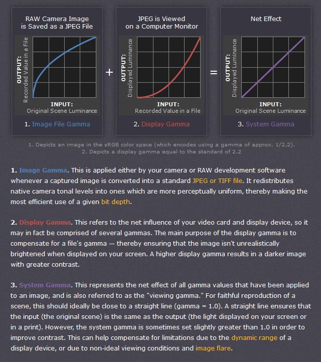
Basically, gamma is the relationship between the brightness of a pixel as it appears on the screen, and the numerical value of that pixel. Generally Gamma is just about defining relationships.
Three main types:
– Image Gamma encoded in images
– Display Gammas encoded in hardware and/or viewing time
– System or Viewing Gamma which is the net effect of all gammas when you look back at a final image. In theory this should flatten back to 1.0 gamma.
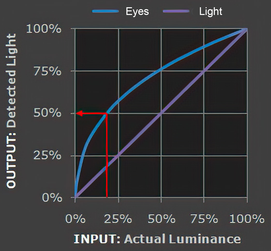
Our eyes, different camera or video recorder devices do not correctly capture luminance. (they are not linear)
Different display devices (monitor, phone screen, TV) do not display luminance correctly neither. So, one needs to correct them, therefore the gamma correction function.
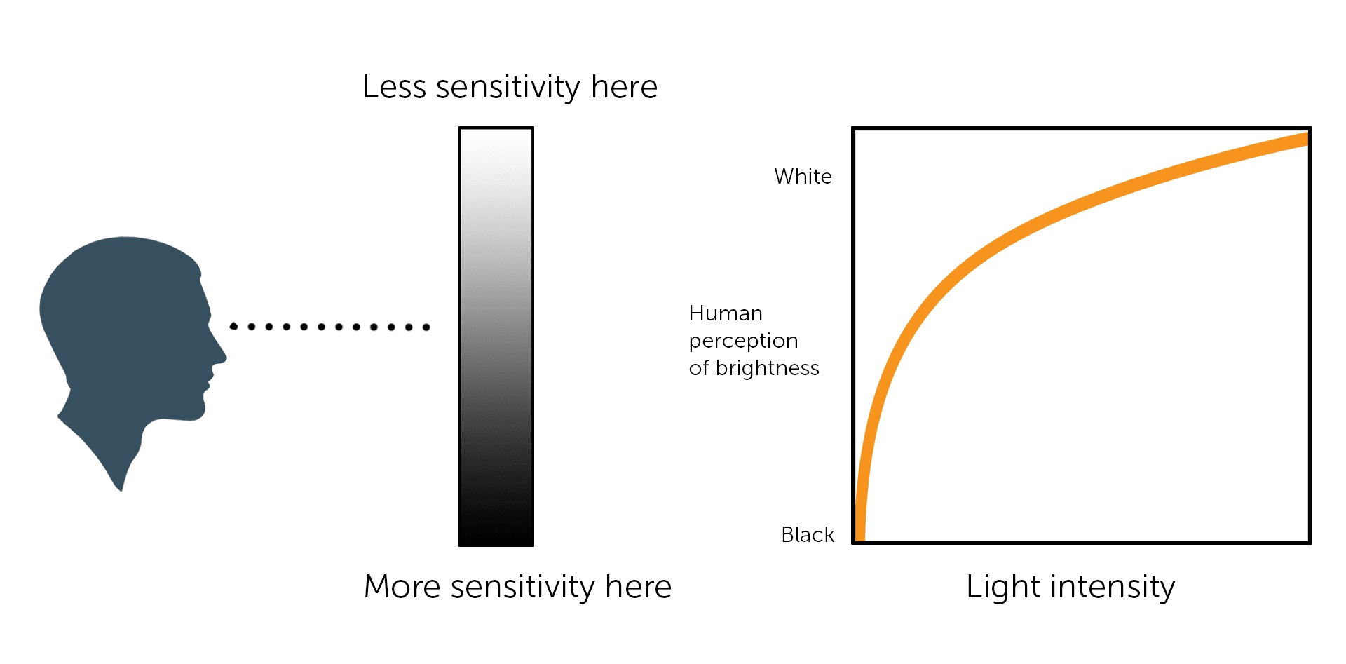
The human perception of brightness, under common illumination conditions (not pitch black nor blindingly bright), follows an approximate power function (note: no relation to the gamma function), with greater sensitivity to relative differences between darker tones than between lighter ones, consistent with the Stevens’ power law for brightness perception. If images are not gamma-encoded, they allocate too many bits or too much bandwidth to highlights that humans cannot differentiate, and too few bits or too little bandwidth to shadow values that humans are sensitive to and would require more bits/bandwidth to maintain the same visual quality.
cones manage color receptivity, rods determine how large our pupils should be. The larger (more dilated) our pupils are, the more light enters our eyes. In dark situations, our rods dilate our pupils so we can see better. This impacts how we perceive brightness.
A gamma encoded image has to have “gamma correction” applied when it is viewed — which effectively converts it back into light from the original scene. In other words, the purpose of gamma encoding is for recording the image — not for displaying the image. Fortunately this second step (the “display gamma”) is automatically performed by your monitor and video card. The following diagram illustrates how all of this fits together:
Display gamma
The display gamma can be a little confusing because this term is often used interchangeably with gamma correction, since it corrects for the file gamma. This is the gamma that you are controlling when you perform monitor calibration and adjust your contrast setting. Fortunately, the industry has converged on a standard display gamma of 2.2, so one doesn’t need to worry about the pros/cons of different values.
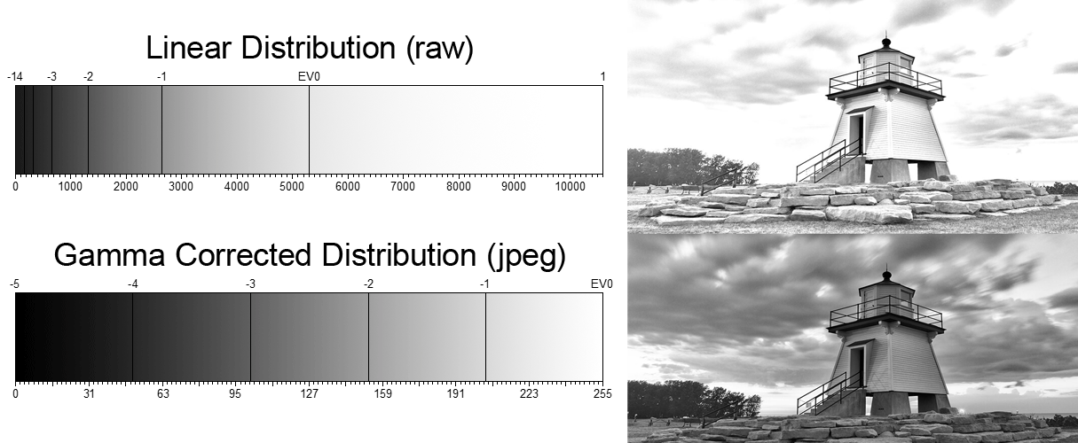
Gamma encoding of images is used to optimize the usage of bits when encoding an image, or bandwidth used to transport an image, by taking advantage of the non-linear manner in which humans perceive light and color. Human response to luminance is also biased. Especially sensible to dark areas.
Thus, the human visual system has a non-linear response to the power of the incoming light, so a fixed increase in power will not have a fixed increase in perceived brightness.
We perceive a value as half bright when it is actually 18% of the original intensity not 50%. As such, our perception is not linear.
You probably already know that a pixel can have any ‘value’ of Red, Green, and Blue between 0 and 255, and you would therefore think that a pixel value of 127 would appear as half of the maximum possible brightness, and that a value of 64 would represent one-quarter brightness, and so on. Well, that’s just not the case.
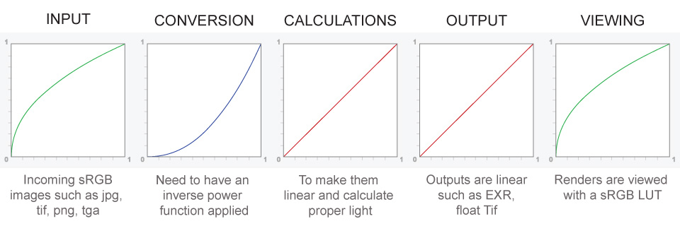
– Why do we need linear gamma?
Because light works linearly and therefore only works properly when it lights linear values.
– Why do we need to view in sRGB?
Because the resulting linear image in not suitable for viewing, but contains all the proper data. Pixar’s IT viewer can compensate by showing the rendered image through a sRGB look up table (LUT), which is identical to what will be the final image after the sRGB gamma curve is applied in post.
This would be simple enough if every software would play by the same rules, but they don’t. In fact, the default gamma workflow for many 3D software is incorrect. This is where the knowledge of a proper imaging workflow comes in to save the day.
Cathode-ray tubes have a peculiar relationship between the voltage applied to them, and the amount of light emitted. It isn’t linear, and in fact it follows what’s called by mathematicians and other geeks, a ‘power law’ (a number raised to a power). The numerical value of that power is what we call the gamma of the monitor or system.
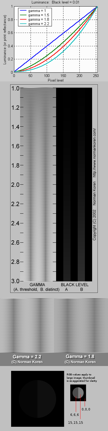
Thus. Gamma describes the nonlinear relationship between the pixel levels in your computer and the luminance of your monitor (the light energy it emits) or the reflectance of your prints. The equation is,
Luminance = C * value^gamma + black level
– C is set by the monitor Contrast control.
– Value is the pixel level normalized to a maximum of 1. For an 8 bit monitor with pixel levels 0 – 255, value = (pixel level)/255.
– Black level is set by the (misnamed) monitor Brightness control. The relationship is linear if gamma = 1. The chart illustrates the relationship for gamma = 1, 1.5, 1.8 and 2.2 with C = 1 and black level = 0.
Gamma affects middle tones; it has no effect on black or white. If gamma is set too high, middle tones appear too dark. Conversely, if it’s set too low, middle tones appear too light.
The native gamma of monitors– the relationship between grid voltage and luminance– is typically around 2.5, though it can vary considerably. This is well above any of the display standards, so you must be aware of gamma and correct it.
A display gamma of 2.2 is the de facto standard for the Windows operating system and the Internet-standard sRGB color space.
The old standard for Mcintosh and prepress file interchange is 1.8. It is now 2.2 as well.
Video cameras have gammas of approximately 0.45– the inverse of 2.2. The viewing or system gamma is the product of the gammas of all the devices in the system– the image acquisition device (film+scanner or digital camera), color lookup table (LUT), and monitor. System gamma is typically between 1.1 and 1.5. Viewing flare and other factor make images look flat at system gamma = 1.0.
Most laptop LCD screens are poorly suited for critical image editing because gamma is extremely sensitive to viewing angle.
CRT Monitors. Due to an odd bit of engineering luck, the native gamma of a CRT is 2.5 — almost the inverse of our eyes. Values from a gamma-encoded file could therefore be sent straight to the screen and they would automatically be corrected and appear nearly OK. However, a small gamma correction of ~1/1.1 needs to be applied to achieve an overall display gamma of 2.2. This is usually already set by the manufacturer’s default settings, but can also be set during monitor calibration.
LCD Monitors. LCD monitors weren’t so fortunate; ensuring an overall display gamma of 2.2 often requires substantial corrections, and they are also much less consistent than CRT’s. LCDs therefore require something called a look-up table (LUT) in order to ensure that input values are depicted using the intended display gamma (amongst other things). See the tutorial on monitor calibration: look-up tables for more on this topic.
About black level (brightness). Your monitor’s brightness control (which should actually be called black level) can be adjusted using the mostly black pattern on the right side of the chart. This pattern contains two dark gray vertical bars, A and B, which increase in luminance with increasing gamma. (If you can’t see them, your black level is way low.) The left bar (A) should be just above the threshold of visibility opposite your chosen gamma (2.2 or 1.8)– it should be invisible where gamma is lower by about 0.3. The right bar (B) should be distinctly visible: brighter than (A), but still very dark. This chart is only for monitors; it doesn’t work on printed media.
The 1.8 and 2.2 gray patterns at the bottom of the image represent a test of monitor quality and calibration. If your monitor is functioning properly and calibrated to gamma = 2.2 or 1.8, the corresponding pattern will appear smooth neutral gray when viewed from a distance. Any waviness, irregularity, or color banding indicates incorrect monitor calibration or poor performance.
Another test to see whether one’s computer monitor is properly hardware adjusted and can display shadow detail in sRGB images properly, they should see the left half of the circle in the large black square very faintly but the right half should be clearly visible. If not, one can adjust their monitor’s contrast and/or brightness setting. This alters the monitor’s perceived gamma. The image is best viewed against a black background.
This procedure is not suitable for calibrating or print-proofing a monitor. It can be useful for making a monitor display sRGB images approximately correctly, on systems in which profiles are not used (for example, the Firefox browser prior to version 3.0 and many others) or in systems that assume untagged source images are in the sRGB colorspace.
On some operating systems running the X Window System, one can set the gamma correction factor (applied to the existing gamma value) by issuing the command xgamma -gamma 0.9 for setting gamma correction factor to 0.9, and xgamma for querying current value of that factor (the default is 1.0). In OS X systems, the gamma and other related screen calibrations are made through the System Preference
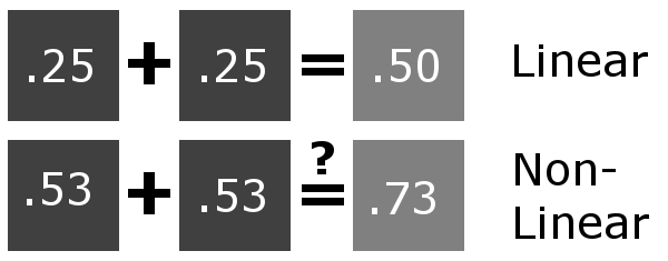
Linear color space means that numerical intensity values correspond proportionally to their perceived intensity. This means that the colors can be added and multiplied correctly. A color space without that property is called ”non-linear”. Below is an example where an intensity value is doubled in a linear and a non-linear color space. While the corresponding numerical values in linear space are correct, in the non-linear space (gamma = 0.45, more on this later) we can’t simply double the value to get the correct intensity.
The need for gamma arises for two main reasons: The first is that screens have been built with a non-linear response to intensity. The other is that the human eye can tell the difference between darker shades better than lighter shades. This means that when images are compressed to save space, we want to have greater accuracy for dark intensities at the expense of lighter intensities. Both of these problems are resolved using gamma correction, which is to say the intensity of every pixel in an image is put through a power function. Specifically, gamma is the name given to the power applied to the image.
CRT screens, simply by how they work, apply a gamma of around 2.2, and modern LCD screens are designed to mimic that behavior. A gamma of 2.2, the reciprocal of 0.45, when applied to the brightened images will darken them, leaving the original image.
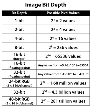
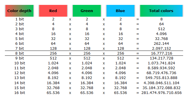
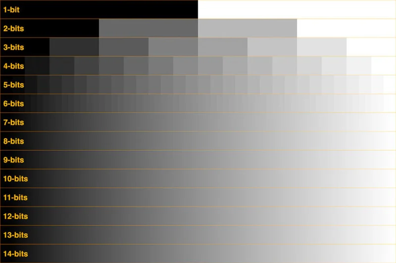
In color technology, color depth also known as bit depth, is either the number of bits used to indicate the color of a single pixel, OR the number of bits used for each color component of a single pixel.
When referring to a pixel, the concept can be defined as bits per pixel (bpp).
When referring to a color component, the concept can be defined as bits per component, bits per channel, bits per color (all three abbreviated bpc), and also bits per pixel component, bits per color channel or bits per sample (bps). Modern standards tend to use bits per component, but historical lower-depth systems used bits per pixel more often.
Color depth is only one aspect of color representation, expressing the precision with which the amount of each primary can be expressed; the other aspect is how broad a range of colors can be expressed (the gamut). The definition of both color precision and gamut is accomplished with a color encoding specification which assigns a digital code value to a location in a color space.
Here’s a simple explanation of each.
8-bit images (i.e. 24 bits per pixel for a color image) are considered Low Dynamic Range. They can store around 5 stops of light and each pixel carry a value from 0 (black) to 255 (white). As a comparison, DSLR cameras can capture ~12-15 stops of light and they use RAW files to store the information.
16-bit: This format is commonly referred to as “half-precision.” It uses 16 bits of data to represent color values for each pixel. With 16 bits, you can have 65,536 discrete levels of color, allowing for relatively high precision and smooth gradients. However, it has a limited dynamic range, meaning it cannot accurately represent extremely bright or dark values. It is commonly used for regular images and textures.
16-bit float: This format is an extension of the 16-bit format but uses floating-point numbers instead of fixed integers. Floating-point numbers allow for more precise calculations and a larger dynamic range. In this case, the 16 bits are used to store both the color value and the exponent, which controls the range of values that can be represented. The 16-bit float format provides better accuracy and a wider dynamic range than regular 16-bit, making it useful for high-dynamic-range imaging (HDRI) and computations that require more precision.
32-bit: (i.e. 96 bits per pixel for a color image) are considered High Dynamic Range. This format, also known as “full-precision” or “float,” uses 32 bits to represent color values and offers the highest precision and dynamic range among the three options. With 32 bits, you have a significantly larger number of discrete levels, allowing for extremely accurate color representation, smooth gradients, and a wide range of brightness values. It is commonly used for professional rendering, visual effects, and scientific applications where maximum precision is required.
Bits and HDR coverage
High Dynamic Range (HDR) images are designed to capture a wide range of luminance values, from the darkest shadows to the brightest highlights, in order to reproduce a scene with more accuracy and detail. The bit depth of an image refers to the number of bits used to represent each pixel’s color information. When comparing 32-bit float and 16-bit float HDR images, the drop in accuracy primarily relates to the precision of the color information.
A 32-bit float HDR image offers a higher level of precision compared to a 16-bit float HDR image. In a 32-bit float format, each color channel (red, green, and blue) is represented by 32 bits, allowing for a larger range of values to be stored. This increased precision enables the image to retain more details and subtleties in color and luminance.
On the other hand, a 16-bit float HDR image utilizes 16 bits per color channel, resulting in a reduced range of values that can be represented. This lower precision leads to a loss of fine details and color nuances, especially in highly contrasted areas of the image where there are significant differences in luminance.
The drop in accuracy between 32-bit and 16-bit float HDR images becomes more noticeable as the exposure range of the scene increases. Exposure range refers to the span between the darkest and brightest areas of an image. In scenes with a limited exposure range, where the luminance differences are relatively small, the loss of accuracy may not be as prominent or perceptible. These images usually are around 8-10 exposure levels.
However, in scenes with a wide exposure range, such as a landscape with deep shadows and bright highlights, the reduced precision of a 16-bit float HDR image can result in visible artifacts like color banding, posterization, and loss of detail in both shadows and highlights. The image may exhibit abrupt transitions between tones or colors, which can appear unnatural and less realistic.
To provide a rough estimate, it is often observed that exposure values beyond approximately ±6 to ±8 stops from the middle gray (18% reflectance) may be more prone to accuracy issues in a 16-bit float format. This range may vary depending on the specific implementation and encoding scheme used.
To summarize, the drop in accuracy between 32-bit and 16-bit float HDR images is mainly related to the reduced precision of color information. This decrease in precision becomes more apparent in scenes with a wide exposure range, affecting the representation of fine details and leading to visible artifacts in the image.
In practice, this means that exposure values beyond a certain range will experience a loss of accuracy and detail when stored in a 16-bit float format. The exact range at which this loss occurs depends on the encoding scheme and the specific implementation. However, in general, extremely bright or extremely dark values that fall outside the representable range may be subject to quantization errors, resulting in loss of detail, banding, or other artifacts.
HDRs used for lighting purposes are usually slightly convolved to improve on sampling speed and removing specular artefacts. To that extent, 16 bit float HDRIs tend to me most used in CG cycles.
Note. The Median Cut algorithm is typically used for color quantization, which involves reducing the number of colors in an image while preserving its visual quality. It doesn’t directly provide a way to identify the brightest areas in an image. However, if you’re interested in identifying the brightest areas, you might want to look into other methods like thresholding, histogram analysis, or edge detection, through openCV for example.
Here is an openCV example:
# bottom left coordinates = 0,0
import numpy as np
import cv2

# Load the HDR or EXR image
image = cv2.imread('your_image_path.exr', cv2.IMREAD_UNCHANGED)  # Load as-is without modification

# Calculate the luminance from the HDR channels (assuming RGB format)
luminance = np.dot(image[..., :3], [0.299, 0.587, 0.114])

# Set a threshold value based on estimated EV
threshold_value = 2.4  # Estimated threshold value based on 4.8 EV

# Apply the threshold to identify bright areas
# The luminance array contains the calculated luminance values for each pixel in the image. # The threshold_value is a user-defined value that represents a cutoff point, separating "bright" and "dark" areas in terms of perceived luminance.
thresholded = (luminance > threshold_value) * 255

# Convert the thresholded image to uint8 for contour detection
thresholded = thresholded.astype(np.uint8)

# Find contours of the bright areas
contours, _ = cv2.findContours(thresholded, cv2.RETR_EXTERNAL, cv2.CHAIN_APPROX_SIMPLE)

# Create a list to store the bounding boxes of bright areas
bright_areas = []

# Iterate through contours and extract bounding boxes for contour in contours:
x, y, w, h = cv2.boundingRect(contour)

# Adjust y-coordinate based on bottom-left origin
y_bottom_left_origin = image.shape[0] - (y + h) bright_areas.append((x, y_bottom_left_origin, x + w, y_bottom_left_origin + h))

# Store as (x1, y1, x2, y2)
# Print the identified bright areas
print("Bright Areas (x1, y1, x2, y2):") for area in bright_areas: print(area)
More details
Luminance and Exposure in an EXR Image:
An EXR (Extended Dynamic Range) image format is often used to store high dynamic range (HDR) images that contain a wide range of luminance values, capturing both dark and bright areas.
Luminance refers to the perceived brightness of a pixel in an image. In an RGB image, luminance is often calculated using a weighted sum of the red, green, and blue channels, where different weights are assigned to each channel to account for human perception.
In an EXR image, the pixel values can represent radiometrically accurate scene values, including actual radiance or irradiance levels. These values are directly related to the amount of light emitted or reflected by objects in the scene.
The luminance line is calculating the luminance of each pixel in the image using a weighted sum of the red, green, and blue channels. The three float values [0.299, 0.587, 0.114] are the weights used to perform this calculation.
These weights are based on the concept of luminosity, which aims to approximate the perceived brightness of a color by taking into account the human eye’s sensitivity to different colors. The values are often derived from the NTSC (National Television System Committee) standard, which is used in various color image processing operations.
Here’s the breakdown of the float values:
0.299: Weight for the red channel.
0.587: Weight for the green channel.
0.114: Weight for the blue channel.
The weighted sum of these channels helps create a grayscale image where the pixel values represent the perceived brightness. This technique is often used when converting a color image to grayscale or when calculating luminance for certain operations, as it takes into account the human eye’s sensitivity to different colors.
For the threshold, remember that the exact relationship between EV values and pixel values can depend on the tone-mapping or normalization applied to the HDR image, as well as the dynamic range of the image itself.
To establish a relationship between exposure and the threshold value, you can consider the relationship between linear and logarithmic scales:
Linear and Logarithmic Scales:
Exposure values in an EXR image are often represented in logarithmic scales, such as EV (exposure value). Each increment in EV represents a doubling or halving of the amount of light captured.
Threshold values for luminance thresholding are usually linear, representing an actual luminance level.
Conversion Between Scales:
To establish a mathematical relationship, you need to convert between the logarithmic exposure scale and the linear threshold scale.
One common method is to use a power function. For instance, you can use a power function to convert EV to a linear intensity value.
threshold_value = base_value * (2 ** EV)
Here, EV is the exposure value, base_value is a scaling factor that determines the relationship between EV and threshold_value, and 2 ** EV is used to convert the logarithmic EV to a linear intensity value.
Choosing the Base Value:
The base_value factor should be determined based on the dynamic range of your EXR image and the specific luminance values you are dealing with.
You may need to experiment with different values of base_value to achieve the desired separation of bright areas from the rest of the image.
Let’s say you have an EXR image with a dynamic range of 12 EV, which is a common range for many high dynamic range images. In this case, you want to set a threshold value that corresponds to a certain number of EV above the middle gray level (which is often considered to be around 0.18).
Here’s an example of how you might determine a base_value to achieve this:
# Define the dynamic range of the image in EV
dynamic_range = 12

# Choose the desired number of EV above middle gray for thresholding
desired_ev_above_middle_gray = 2

# Calculate the threshold value based on the desired EV above middle gray
threshold_value = 0.18 * (2 ** (desired_ev_above_middle_gray / dynamic_range))

print("Threshold Value:", threshold_value)
In general, when light interacts with matter, a complicated light-matter dynamic occurs. This interaction depends on the physical characteristics of the light as well as the physical composition and characteristics of the matter.
That is, some of the incident light is reflected, some of the light is transmitted, and another portion of the light is absorbed by the medium itself.
A BRDF describes how much light is reflected when light makes contact with a certain material. Similarly, a BTDF (Bi-directional Transmission Distribution Function) describes how much light is transmitted when light makes contact with a certain material
It is difficult to establish exactly how far one should go in elaborating the surface model. A truly complete representation of the reflective behavior of a surface might take into account such phenomena as polarization, scattering, fluorescence, and phosphorescence, all of which might vary with position on the surface. Therefore, the variables in this complete function would be:
incoming and outgoing angle incoming and outgoing wavelength incoming and outgoing polarization (both linear and circular) incoming and outgoing position (which might differ due to subsurface scattering) time delay between the incoming and outgoing light ray
As Einstein showed us, light and matter and just aspects of the same thing. Matter is just frozen light. And light is matter on the move. Albert Einstein’s most famous equation says that energy and matter are two sides of the same coin. How does one become the other?
Relativity requires that the faster an object moves, the more mass it appears to have. This means that somehow part of the energy of the car’s motion appears to transform into mass. Hence the origin of Einstein’s equation. How does that happen? We don’t really know. We only know that it does.
Matter is 99.999999999999 percent empty space. Not only do the atom and solid matter consist mainly of empty space, it is the same in outer space
The quantum theory researchers discovered the answer: Not only do particles consist of energy, but so does the space between. This is the so-called zero-point energy. Therefore it is true: Everything consists of energy.
Energy is the basis of material reality. Every type of particle is conceived of as a quantum vibration in a field: Electrons are vibrations in electron fields, protons vibrate in a proton field, and so on. Everything is energy, and everything is connected to everything else through fields.
DISCLAIMER – Links and images on this website may be protected by the respective owners’ copyright. All data submitted by users through this site shall be treated as freely available to share.