


COMPOSITION
-
Photography basics: Depth of Field and composition
Read more: Photography basics: Depth of Field and compositionDepth of field is the range within which focusing is resolved in a photo.
Aperture has a huge affect on to the depth of field.
Changing the f-stops (f/#) of a lens will change aperture and as such the DOF.
f-stops are a just certain number which is telling you the size of the aperture. That’s how f-stop is related to aperture (and DOF).
If you increase f-stops, it will increase DOF, the area in focus (and decrease the aperture). On the other hand, decreasing the f-stop it will decrease DOF (and increase the aperture).
The red cone in the figure is an angular representation of the resolution of the system. Versus the dotted lines, which indicate the aperture coverage. Where the lines of the two cones intersect defines the total range of the depth of field.
This image explains why the longer the depth of field, the greater the range of clarity.


DESIGN


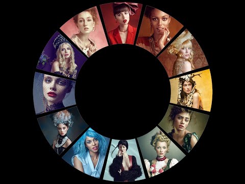
COLOR
-
Photography basics: Why Use a (MacBeth) Color Chart?
Read more: Photography basics: Why Use a (MacBeth) Color Chart?Start here: https://www.pixelsham.com/2013/05/09/gretagmacbeth-color-checker-numeric-values/
https://www.studiobinder.com/blog/what-is-a-color-checker-tool/


In LightRoom

in Final Cut

in Nuke
Note: In Foundry’s Nuke, the software will map 18% gray to whatever your center f/stop is set to in the viewer settings (f/8 by default… change that to EV by following the instructions below).
You can experiment with this by attaching an Exposure node to a Constant set to 0.18, setting your viewer read-out to Spotmeter, and adjusting the stops in the node up and down. You will see that a full stop up or down will give you the respective next value on the aperture scale (f8, f11, f16 etc.).One stop doubles or halves the amount or light that hits the filmback/ccd, so everything works in powers of 2.
So starting with 0.18 in your constant, you will see that raising it by a stop will give you .36 as a floating point number (in linear space), while your f/stop will be f/11 and so on.If you set your center stop to 0 (see below) you will get a relative readout in EVs, where EV 0 again equals 18% constant gray.

In other words. Setting the center f-stop to 0 means that in a neutral plate, the middle gray in the macbeth chart will equal to exposure value 0. EV 0 corresponds to an exposure time of 1 sec and an aperture of f/1.0.
This will set the sun usually around EV12-17 and the sky EV1-4 , depending on cloud coverage.
To switch Foundry’s Nuke’s SpotMeter to return the EV of an image, click on the main viewport, and then press s, this opens the viewer’s properties. Now set the center f-stop to 0 in there. And the SpotMeter in the viewport will change from aperture and fstops to EV.
-
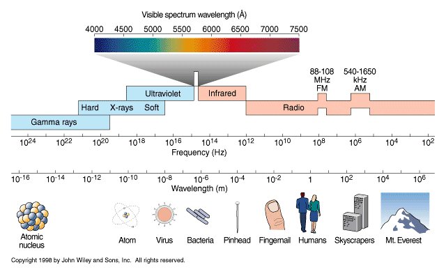
Sensitivity of human eye
Read more: Sensitivity of human eyehttp://www.wikilectures.eu/index.php/Spectral_sensitivity_of_the_human_eye
http://www.normankoren.com/Human_spectral_sensitivity_small.jpg
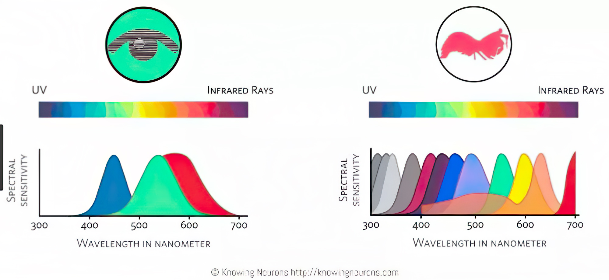
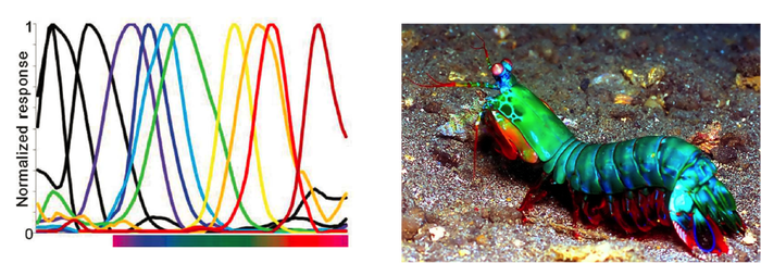
Spectral sensitivity of eye is influenced by light intensity. And the light intensity determines the level of activity of cones cell and rod cell. This is the main characteristic of human vision. Sensitivity to individual colors, in other words, wavelengths of the light spectrum, is explained by the RGB (red-green-blue) theory. This theory assumed that there are three kinds of cones. It’s selectively sensitive to red (700-630 nm), green (560-500 nm), and blue (490-450 nm) light. And their mutual interaction allow to perceive all colors of the spectrum.
http://weeklysciencequiz.blogspot.com/2013/01/violet-skies-are-for-birds.html

Sensitivity of human eye Sensitivity of human eyes to light increase with the decrease in light intensity. In day-light condition, the cones cell is responding to this condition. And the eye is most sensitive at 555 nm. In darkness condition, the rod cell is responding to this condition. And the eye is most sensitive at 507 nm.
As light intensity decreases, cone function changes more effective way. And when decrease the light intensity, it prompt to accumulation of rhodopsin. Furthermore, in activates rods, it allow to respond to stimuli of light in much lower intensity.
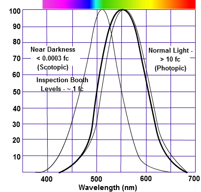
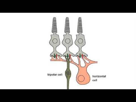
The three curves in the figure above shows the normalized response of an average human eye to various amounts of ambient light. The shift in sensitivity occurs because two types of photoreceptors called cones and rods are responsible for the eye’s response to light. The curve on the right shows the eye’s response under normal lighting conditions and this is called the photopic response. The cones respond to light under these conditions.
As mentioned previously, cones are composed of three different photo pigments that enable color perception. This curve peaks at 555 nanometers, which means that under normal lighting conditions, the eye is most sensitive to a yellowish-green color. When the light levels drop to near total darkness, the response of the eye changes significantly as shown by the scotopic response curve on the left. At this level of light, the rods are most active and the human eye is more sensitive to the light present, and less sensitive to the range of color. Rods are highly sensitive to light but are comprised of a single photo pigment, which accounts for the loss in ability to discriminate color. At this very low light level, sensitivity to blue, violet, and ultraviolet is increased, but sensitivity to yellow and red is reduced. The heavier curve in the middle represents the eye’s response at the ambient light level found in a typical inspection booth. This curve peaks at 550 nanometers, which means the eye is most sensitive to yellowish-green color at this light level. Fluorescent penetrant inspection materials are designed to fluoresce at around 550 nanometers to produce optimal sensitivity under dim lighting conditions.
-
Weta Digital – Manuka Raytracer and Gazebo GPU renderers – pipeline
Read more: Weta Digital – Manuka Raytracer and Gazebo GPU renderers – pipelinehttps://jo.dreggn.org/home/2018_manuka.pdf
http://www.fxguide.com/featured/manuka-weta-digitals-new-renderer/

The Manuka rendering architecture has been designed in the spirit of the classic reyes rendering architecture. In its core, reyes is based on stochastic rasterisation of micropolygons, facilitating depth of field, motion blur, high geometric complexity,and programmable shading.
This is commonly achieved with Monte Carlo path tracing, using a paradigm often called shade-on-hit, in which the renderer alternates tracing rays with running shaders on the various ray hits. The shaders take the role of generating the inputs of the local material structure which is then used bypath sampling logic to evaluate contributions and to inform what further rays to cast through the scene.
Over the years, however, the expectations have risen substantially when it comes to image quality. Computing pictures which are indistinguishable from real footage requires accurate simulation of light transport, which is most often performed using some variant of Monte Carlo path tracing. Unfortunately this paradigm requires random memory accesses to the whole scene and does not lend itself well to a rasterisation approach at all.
Manuka is both a uni-directional and bidirectional path tracer and encompasses multiple importance sampling (MIS). Interestingly, and importantly for production character skin work, it is the first major production renderer to incorporate spectral MIS in the form of a new ‘Hero Spectral Sampling’ technique, which was recently published at Eurographics Symposium on Rendering 2014.
Manuka propose a shade-before-hit paradigm in-stead and minimise I/O strain (and some memory costs) on the system, leveraging locality of reference by running pattern generation shaders before we execute light transport simulation by path sampling, “compressing” any bvh structure as needed, and as such also limiting duplication of source data.
The difference with reyes is that instead of baking colors into the geometry like in Reyes, manuka bakes surface closures. This means that light transport is still calculated with path tracing, but all texture lookups etc. are done up-front and baked into the geometry.The main drawback with this method is that geometry has to be tessellated to its highest, stable topology before shading can be evaluated properly. As such, the high cost to first pixel. Even a basic 4 vertices square becomes a much more complex model with this approach.

Manuka use the RenderMan Shading Language (rsl) for programmable shading [Pixar Animation Studios 2015], but we do not invoke rsl shaders when intersecting a ray with a surface (often called shade-on-hit). Instead, we pre-tessellate and pre-shade all the input geometry in the front end of the renderer.
This way, we can efficiently order shading computations to sup-port near-optimal texture locality, vectorisation, and parallelism. This system avoids repeated evaluation of shaders at the same surface point, and presents a minimal amount of memory to be accessed during light transport time. An added benefit is that the acceleration structure for ray tracing (abounding volume hierarchy, bvh) is built once on the final tessellated geometry, which allows us to ray trace more efficiently than multi-level bvhs and avoids costly caching of on-demand tessellated micropolygons and the associated scheduling issues.For the shading reasons above, in terms of AOVs, the studio approach is to succeed at combining complex shading with ray paths in the render rather than pass a multi-pass render to compositing.
For the Spectral Rendering component. The light transport stage is fully spectral, using a continuously sampled wavelength which is traced with each path and used to apply the spectral camera sensitivity of the sensor. This allows for faithfully support any degree of observer metamerism as the camera footage they are intended to match as well as complex materials which require wavelength dependent phenomena such as diffraction, dispersion, interference, iridescence, or chromatic extinction and Rayleigh scattering in participating media.
As opposed to the original reyes paper, we use bilinear interpolation of these bsdf inputs later when evaluating bsdfs per pathv ertex during light transport4. This improves temporal stability of geometry which moves very slowly with respect to the pixel raster
In terms of the pipeline, everything rendered at Weta was already completely interwoven with their deep data pipeline. Manuka very much was written with deep data in mind. Here, Manuka not so much extends the deep capabilities, rather it fully matches the already extremely complex and powerful setup Weta Digital already enjoy with RenderMan. For example, an ape in a scene can be selected, its ID is available and a NUKE artist can then paint in 3D say a hand and part of the way up the neutral posed ape.
We called our system Manuka, as a respectful nod to reyes: we had heard a story froma former ILM employee about how reyes got its name from how fond the early Pixar people were of their lunches at Point Reyes, and decided to name our system after our surrounding natural environment, too. Manuka is a kind of tea tree very common in New Zealand which has very many very small leaves, in analogy to micropolygons ina tree structure for ray tracing. It also happens to be the case that Weta Digital’s main site is on Manuka Street.

-
Space bodies’ components and light spectroscopy
Read more: Space bodies’ components and light spectroscopywww.plutorules.com/page-111-space-rocks.html
This help’s us understand the composition of components in/on solar system bodies.
Dips in the observed light spectrum, also known as, lines of absorption occur as gasses absorb energy from light at specific points along the light spectrum.
These dips or darkened zones (lines of absorption) leave a finger print which identify elements and compounds.
In this image the dark absorption bands appear as lines of emission which occur as the result of emitted not reflected (absorbed) light.
Lines of absorption
 Lines of emission


-
Björn Ottosson – OKHSV and OKHSL – Two new color spaces for color picking
Read more: Björn Ottosson – OKHSV and OKHSL – Two new color spaces for color pickinghttps://bottosson.github.io/misc/colorpicker
https://bottosson.github.io/posts/colorpicker/
https://www.smashingmagazine.com/2024/10/interview-bjorn-ottosson-creator-oklab-color-space/
One problem with sRGB is that in a gradient between blue and white, it becomes a bit purple in the middle of the transition. That’s because sRGB really isn’t created to mimic how the eye sees colors; rather, it is based on how CRT monitors work. That means it works with certain frequencies of red, green, and blue, and also the non-linear coding called gamma. It’s a miracle it works as well as it does, but it’s not connected to color perception. When using those tools, you sometimes get surprising results, like purple in the gradient.

There were also attempts to create simple models matching human perception based on XYZ, but as it turned out, it’s not possible to model all color vision that way. Perception of color is incredibly complex and depends, among other things, on whether it is dark or light in the room and the background color it is against. When you look at a photograph, it also depends on what you think the color of the light source is. The dress is a typical example of color vision being very context-dependent. It is almost impossible to model this perfectly.
I based Oklab on two other color spaces, CIECAM16 and IPT. I used the lightness and saturation prediction from CIECAM16, which is a color appearance model, as a target. I actually wanted to use the datasets used to create CIECAM16, but I couldn’t find them.
IPT was designed to have better hue uniformity. In experiments, they asked people to match light and dark colors, saturated and unsaturated colors, which resulted in a dataset for which colors, subjectively, have the same hue. IPT has a few other issues but is the basis for hue in Oklab.
In the Munsell color system, colors are described with three parameters, designed to match the perceived appearance of colors: Hue, Chroma and Value. The parameters are designed to be independent and each have a uniform scale. This results in a color solid with an irregular shape. The parameters are designed to be independent and each have a uniform scale. This results in a color solid with an irregular shape. Modern color spaces and models, such as CIELAB, Cam16 and Björn Ottosson own Oklab, are very similar in their construction.

By far the most used color spaces today for color picking are HSL and HSV, two representations introduced in the classic 1978 paper “Color Spaces for Computer Graphics”. HSL and HSV designed to roughly correlate with perceptual color properties while being very simple and cheap to compute.
Today HSL and HSV are most commonly used together with the sRGB color space.

One of the main advantages of HSL and HSV over the different Lab color spaces is that they map the sRGB gamut to a cylinder. This makes them easy to use since all parameters can be changed independently, without the risk of creating colors outside of the target gamut.

The main drawback on the other hand is that their properties don’t match human perception particularly well.
Reconciling these conflicting goals perfectly isn’t possible, but given that HSV and HSL don’t use anything derived from experiments relating to human perception, creating something that makes a better tradeoff does not seem unreasonable.
With this new lightness estimate, we are ready to look into the construction of Okhsv and Okhsl.


-
VES Cinematic Color – Motion-Picture Color Management
Read more: VES Cinematic Color – Motion-Picture Color ManagementThis paper presents an introduction to the color pipelines behind modern feature-film visual-effects and animation.
Authored by Jeremy Selan, and reviewed by the members of the VES Technology Committee including Rob Bredow, Dan Candela, Nick Cannon, Paul Debevec, Ray Feeney, Andy Hendrickson, Gautham Krishnamurti, Sam Richards, Jordan Soles, and Sebastian Sylwan.


LIGHTING
-
Open Source Nvidia Omniverse
Read more: Open Source Nvidia Omniverseblogs.nvidia.com/blog/2019/03/18/omniverse-collaboration-platform/

developer.nvidia.com/nvidia-omniverse
An open, Interactive 3D Design Collaboration Platform for Multi-Tool Workflows to simplify studio workflows for real-time graphics.
It supports Pixar’s Universal Scene Description technology for exchanging information about modeling, shading, animation, lighting, visual effects and rendering across multiple applications.
It also supports NVIDIA’s Material Definition Language, which allows artists to exchange information about surface materials across multiple tools.
With Omniverse, artists can see live updates made by other artists working in different applications. They can also see changes reflected in multiple tools at the same time.
For example an artist using Maya with a portal to Omniverse can collaborate with another artist using UE4 and both will see live updates of each others’ changes in their application.
-
Neural Microfacet Fields for Inverse Rendering
Read more: Neural Microfacet Fields for Inverse Renderinghttps://half-potato.gitlab.io/posts/nmf/

-
Magnific.ai Relight – change the entire lighting of a scene
Read more: Magnific.ai Relight – change the entire lighting of a scene
It’s a new Magnific spell that allows you to change the entire lighting of a scene and, optionally, the background with just:
1/ A prompt OR
2/ A reference image OR
3/ A light map (drawing your own lights)https://x.com/javilopen/status/1805274155065176489


-
Rendering – BRDF – Bidirectional reflectance distribution function
Read more: Rendering – BRDF – Bidirectional reflectance distribution functionhttp://en.wikipedia.org/wiki/Bidirectional_reflectance_distribution_function
The bidirectional reflectance distribution function is a four-dimensional function that defines how light is reflected at an opaque surface
http://www.cs.ucla.edu/~zhu/tutorial/An_Introduction_to_BRDF-Based_Lighting.pdf
In general, when light interacts with matter, a complicated light-matter dynamic occurs. This interaction depends on the physical characteristics of the light as well as the physical composition and characteristics of the matter.
That is, some of the incident light is reflected, some of the light is transmitted, and another portion of the light is absorbed by the medium itself.
A BRDF describes how much light is reflected when light makes contact with a certain material. Similarly, a BTDF (Bi-directional Transmission Distribution Function) describes how much light is transmitted when light makes contact with a certain material
http://www.cs.princeton.edu/~smr/cs348c-97/surveypaper.html
It is difficult to establish exactly how far one should go in elaborating the surface model. A truly complete representation of the reflective behavior of a surface might take into account such phenomena as polarization, scattering, fluorescence, and phosphorescence, all of which might vary with position on the surface. Therefore, the variables in this complete function would be:
incoming and outgoing angle incoming and outgoing wavelength incoming and outgoing polarization (both linear and circular) incoming and outgoing position (which might differ due to subsurface scattering) time delay between the incoming and outgoing light ray


COLLECTIONS
| Featured AI
| Design And Composition
| Explore posts
POPULAR SEARCHES
unreal | pipeline | virtual production | free | learn | photoshop | 360 | macro | google | nvidia | resolution | open source | hdri | real-time | photography basics | nuke
FEATURED POSTS
-
The Perils of Technical Debt – Understanding Its Impact on Security, Usability, and Stability
-
Image rendering bit depth
-
Python and TCL: Tips and Tricks for Foundry Nuke
-
Want to build a start up company that lasts? Think three-layer cake
-
Photography basics: Lumens vs Candelas (candle) vs Lux vs FootCandle vs Watts vs Irradiance vs Illuminance
-
RawTherapee – a free, open source, cross-platform raw image and HDRi processing program
-
MiniMax-Remover – Taming Bad Noise Helps Video Object Removal Rotoscoping
-
N8N.io – From Zero to Your First AI Agent in 25 Minutes
Social Links
DISCLAIMER – Links and images on this website may be protected by the respective owners’ copyright. All data submitted by users through this site shall be treated as freely available to share.
