


COMPOSITION
-
HuggingFace ai-comic-factory – a FREE AI Comic Book Creator
Read more: HuggingFace ai-comic-factory – a FREE AI Comic Book Creatorhttps://huggingface.co/spaces/jbilcke-hf/ai-comic-factory

this is the epic story of a group of talented digital artists trying to overcame daily technical challenges to achieve incredibly photorealistic projects of monsters and aliens


DESIGN
COLOR
-
Light and Matter : The 2018 theory of Physically-Based Rendering and Shading by Allegorithmic
Read more: Light and Matter : The 2018 theory of Physically-Based Rendering and Shading by Allegorithmicacademy.substance3d.com/courses/the-pbr-guide-part-1
academy.substance3d.com/courses/the-pbr-guide-part-2

 Local copy:
-
Pattern generators
Read more: Pattern generatorshttp://qrohlf.com/trianglify-generator/
https://halftonepro.com/app/polygons#
https://mattdesl.svbtle.com/generative-art-with-nodejs-and-canvas
https://www.patterncooler.com/
http://permadi.com/java/spaint/spaint.html
https://dribbble.com/shots/1847313-Kaleidoscope-Generator-PSD
http://eskimoblood.github.io/gerstnerizer/
http://www.stripegenerator.com/
http://btmills.github.io/geopattern/geopattern.html
http://fractalarchitect.net/FA4-Random-Generator.html
https://sciencevsmagic.net/fractal/#0605,0000,3,2,0,1,2
https://sites.google.com/site/mandelbulber/home
-
Photography basics: Why Use a (MacBeth) Color Chart?
Read more: Photography basics: Why Use a (MacBeth) Color Chart?Start here: https://www.pixelsham.com/2013/05/09/gretagmacbeth-color-checker-numeric-values/
https://www.studiobinder.com/blog/what-is-a-color-checker-tool/


In LightRoom

in Final Cut

in Nuke
Note: In Foundry’s Nuke, the software will map 18% gray to whatever your center f/stop is set to in the viewer settings (f/8 by default… change that to EV by following the instructions below).
You can experiment with this by attaching an Exposure node to a Constant set to 0.18, setting your viewer read-out to Spotmeter, and adjusting the stops in the node up and down. You will see that a full stop up or down will give you the respective next value on the aperture scale (f8, f11, f16 etc.).One stop doubles or halves the amount or light that hits the filmback/ccd, so everything works in powers of 2.
So starting with 0.18 in your constant, you will see that raising it by a stop will give you .36 as a floating point number (in linear space), while your f/stop will be f/11 and so on.If you set your center stop to 0 (see below) you will get a relative readout in EVs, where EV 0 again equals 18% constant gray.

In other words. Setting the center f-stop to 0 means that in a neutral plate, the middle gray in the macbeth chart will equal to exposure value 0. EV 0 corresponds to an exposure time of 1 sec and an aperture of f/1.0.
This will set the sun usually around EV12-17 and the sky EV1-4 , depending on cloud coverage.
To switch Foundry’s Nuke’s SpotMeter to return the EV of an image, click on the main viewport, and then press s, this opens the viewer’s properties. Now set the center f-stop to 0 in there. And the SpotMeter in the viewport will change from aperture and fstops to EV.
-
PTGui 13 beta adds control through a Patch Editor
Read more: PTGui 13 beta adds control through a Patch EditorAdditions:
- Patch Editor (PTGui Pro)
- DNG output
- Improved RAW / DNG handling
- JPEG 2000 support
- Performance improvements

-
FXGuide – ACES 2.0 with ILM’s Alex Fry
Read more: FXGuide – ACES 2.0 with ILM’s Alex Fry
https://draftdocs.acescentral.com/background/whats-new/
ACES 2.0 is the second major release of the components that make up the ACES system. The most significant change is a new suite of rendering transforms whose design was informed by collected feedback and requests from users of ACES 1. The changes aim to improve the appearance of perceived artifacts and to complete previously unfinished components of the system, resulting in a more complete, robust, and consistent product.
Highlights of the key changes in ACES 2.0 are as follows:
- New output transforms, including:
- A less aggressive tone scale
- More intuitive controls to create custom outputs to non-standard displays
- Robust gamut mapping to improve perceptual uniformity
- Improved performance of the inverse transforms
- Enhanced AMF specification
- An updated specification for ACES Transform IDs
- OpenEXR compression recommendations
- Enhanced tools for generating Input Transforms and recommended procedures for characterizing prosumer cameras
- Look Transform Library
- Expanded documentation
Rendering Transform
The most substantial change in ACES 2.0 is a complete redesign of the rendering transform.
ACES 2.0 was built as a unified system, rather than through piecemeal additions. Different deliverable outputs “match” better and making outputs to display setups other than the provided presets is intended to be user-driven. The rendering transforms are less likely to produce undesirable artifacts “out of the box”, which means less time can be spent fixing problematic images and more time making pictures look the way you want.
Key design goals
- Improve consistency of tone scale and provide an easy to use parameter to allow for outputs between preset dynamic ranges
- Minimize hue skews across exposure range in a region of same hue
- Unify for structural consistency across transform type
- Easy to use parameters to create outputs other than the presets
- Robust gamut mapping to improve harsh clipping artifacts
- Fill extents of output code value cube (where appropriate and expected)
- Invertible – not necessarily reversible, but Output > ACES > Output round-trip should be possible
- Accomplish all of the above while maintaining an acceptable “out-of-the box” rendering
- New output transforms, including:
-
No one could see the colour blue until modern times
Read more: No one could see the colour blue until modern timeshttps://www.businessinsider.com/what-is-blue-and-how-do-we-see-color-2015-2

The way that humans see the world… until we have a way to describe something, even something so fundamental as a colour, we may not even notice that something it’s there.
Ancient languages didn’t have a word for blue — not Greek, not Chinese, not Japanese, not Hebrew, not Icelandic cultures. And without a word for the colour, there’s evidence that they may not have seen it at all.
https://www.wnycstudios.org/story/211119-colors
Every language first had a word for black and for white, or dark and light. The next word for a colour to come into existence — in every language studied around the world — was red, the colour of blood and wine.
After red, historically, yellow appears, and later, green (though in a couple of languages, yellow and green switch places). The last of these colours to appear in every language is blue.
The only ancient culture to develop a word for blue was the Egyptians — and as it happens, they were also the only culture that had a way to produce a blue dye.
https://mymodernmet.com/shades-of-blue-color-history/
https://www.msn.com/en-us/news/technology/scientists-recreate-lost-recipes-for-a-5-000-year-old-egyptian-blue-dye/ar-AA1FXcj1
Assessment of process variability and color in synthesized and ancient Egyptian blue pigments | npj Heritage ScienceThe approximately 5,000-year-old dye wasn’t a single color, but instead encompassed a range of hues, from deep blues to duller grays and greens. Artisans first crafted Egyptian blue during the Fourth Dynasty (roughly 2613 to 2494 BCE) from recipes reliant on calcium-copper silicate. These techniques were later adopted by Romans in lieu of more expensive materials like lapis lazuli and turquoise. But the additional ingredient lists were lost to history by the time of the Renaissance.
McCloy’s team confirmed that cuprorivaite—the naturally occurring mineral equivalent to Egyptian blue—remains the primary color influence in each hue. Despite the presence of other components, Egyptian blue appears as a uniform color after the cuprorivaite becomes encased in colorless particles such as silicate during the heating process.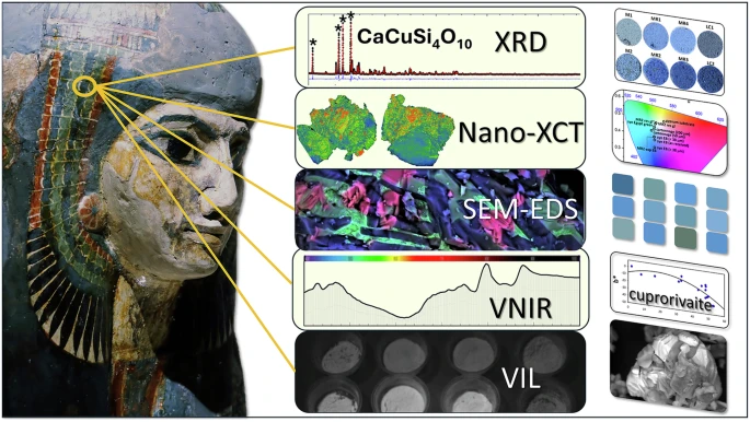
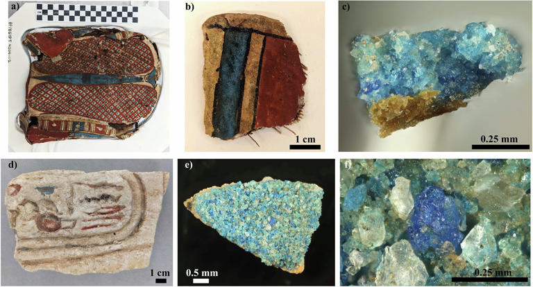
Considered to be the first ever synthetically produced color pigment, Egyptian blue (also known as cuprorivaite) was created around 2,200 B.C. It was made from ground limestone mixed with sand and a copper-containing mineral, such as azurite or malachite, which was then heated between 1470 and 1650°F. The result was an opaque blue glass which then had to be crushed and combined with thickening agents such as egg whites to create a long-lasting paint or glaze.
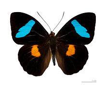
If you think about it, blue doesn’t appear much in nature — there aren’t animals with blue pigments (except for one butterfly, Obrina Olivewing, all animals generate blue through light scattering), blue eyes are rare (also blue through light scattering), and blue flowers are mostly human creations. There is, of course, the sky, but is that really blue?

So before we had a word for it, did people not naturally see blue? Do you really see something if you don’t have a word for it?
A researcher named Jules Davidoff traveled to Namibia to investigate this, where he conducted an experiment with the Himba tribe, who speak a language that has no word for blue or distinction between blue and green. When shown a circle with 11 green squares and one blue, they couldn’t pick out which one was different from the others.
When looking at a circle of green squares with only one slightly different shade, they could immediately spot the different one. Can you?
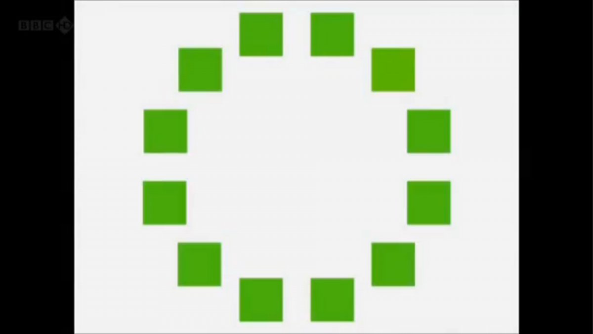
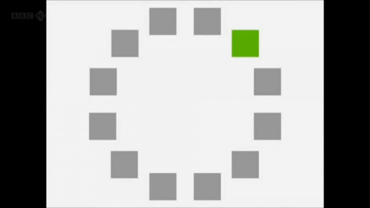
Davidoff says that without a word for a colour, without a way of identifying it as different, it’s much harder for us to notice what’s unique about it — even though our eyes are physically seeing the blocks it in the same way.
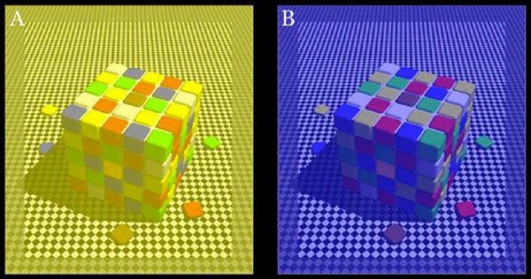
Further research brought to wider discussions about color perception in humans. Everything that we make is based on the fact that humans are trichromatic. The television only has 3 colors. Our color printers have 3 different colors. But some people, and in specific some women seemed to be more sensible to color differences… mainly because they’re just more aware or – because of the job that they do.
Eventually this brought to the discovery of a small percentage of the population, referred to as tetrachromats, which developed an extra cone sensitivity to yellow, likely due to gene modifications.
The interesting detail about these is that even between tetrachromats, only the ones that had a reason to develop, label and work with extra color sensitivity actually developed the ability to use their native skills.
So before blue became a common concept, maybe humans saw it. But it seems they didn’t know they were seeing it.
If you see something yet can’t see it, does it exist? Did colours come into existence over time? Not technically, but our ability to notice them… may have…
-
Photography basics: Lumens vs Candelas (candle) vs Lux vs FootCandle vs Watts vs Irradiance vs Illuminance
Read more: Photography basics: Lumens vs Candelas (candle) vs Lux vs FootCandle vs Watts vs Irradiance vs Illuminancehttps://www.translatorscafe.com/unit-converter/en-US/illumination/1-11/

The power output of a light source is measured using the unit of watts W. This is a direct measure to calculate how much power the light is going to drain from your socket and it is not relatable to the light brightness itself.
The amount of energy emitted from it per second. That energy comes out in a form of photons which we can crudely represent with rays of light coming out of the source. The higher the power the more rays emitted from the source in a unit of time.
Not all energy emitted is visible to the human eye, so we often rely on photometric measurements, which takes in account the sensitivity of human eye to different wavelenghts


Details in the post
(more…)


LIGHTING
-
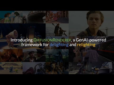
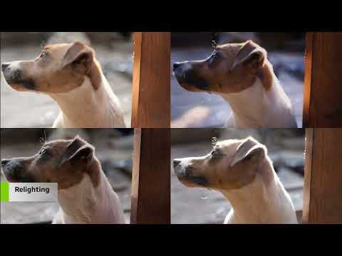
NVidia DiffusionRenderer – Neural Inverse and Forward Rendering with Video Diffusion Models. How NVIDIA reimagined relighting
Read more: NVidia DiffusionRenderer – Neural Inverse and Forward Rendering with Video Diffusion Models. How NVIDIA reimagined relightinghttps://www.fxguide.com/quicktakes/diffusing-reality-how-nvidia-reimagined-relighting/
https://research.nvidia.com/labs/toronto-ai/DiffusionRenderer/
-
About green screens
Read more: About green screenshackaday.com/2015/02/07/how-green-screen-worked-before-computers/
www.newtek.com/blog/tips/best-green-screen-materials/
www.chromawall.com/blog//chroma-key-green

Chroma Key Green, the color of green screens is also known as Chroma Green and is valued at approximately 354C in the Pantone color matching system (PMS).
Chroma Green can be broken down in many different ways. Here is green screen green as other values useful for both physical and digital production:
Green Screen as RGB Color Value: 0, 177, 64
Green Screen as CMYK Color Value: 81, 0, 92, 0
Green Screen as Hex Color Value: #00b140
Green Screen as Websafe Color Value: #009933Chroma Key Green is reasonably close to an 18% gray reflectance.
Illuminate your green screen with an uniform source with less than 2/3 EV variation.
The level of brightness at any given f-stop should be equivalent to a 90% white card under the same lighting. -
Vahan Sosoyan MakeHDR – an OpenFX open source plug-in for merging multiple LDR images into a single HDRI
Read more: Vahan Sosoyan MakeHDR – an OpenFX open source plug-in for merging multiple LDR images into a single HDRIhttps://github.com/Sosoyan/make-hdr
Feature notes
- Merge up to 16 inputs with 8, 10 or 12 bit depth processing
- User friendly logarithmic Tone Mapping controls within the tool
- Advanced controls such as Sampling rate and Smoothness
Available at cross platform on Linux, MacOS and Windows Works consistent in compositing applications like Nuke, Fusion, Natron.
NOTE: The goal is to clean the initial individual brackets before or at merging time as much as possible.
This means:- keeping original shooting metadata
- de-fringing
- removing aberration (through camera lens data or automatically)
- at 32 bit
- in ACEScg (or ACES) wherever possible

-
Bella – Fast Spectral Rendering
Read more: Bella – Fast Spectral Rendering
Bella works in spectral space, allowing effects such as BSDF wavelength dependency, diffraction, or atmosphere to be modeled far more accurately than in color space.

https://superrendersfarm.com/blog/uncategorized/bella-a-new-spectral-physically-based-renderer/
-
Sun cone angle (angular diameter) as perceived by earth viewers
Read more: Sun cone angle (angular diameter) as perceived by earth viewersAlso see:
https://www.pixelsham.com/2020/08/01/solid-angle-measures/
The cone angle of the sun refers to the angular diameter of the sun as observed from Earth, which is related to the apparent size of the sun in the sky.
The angular diameter of the sun, or the cone angle of the sunlight as perceived from Earth, is approximately 0.53 degrees on average. This value can vary slightly due to the elliptical nature of Earth’s orbit around the sun, but it generally stays within a narrow range.
Here’s a more precise breakdown:
-
- Average Angular Diameter: About 0.53 degrees (31 arcminutes)
- Minimum Angular Diameter: Approximately 0.52 degrees (when Earth is at aphelion, the farthest point from the sun)
- Maximum Angular Diameter: Approximately 0.54 degrees (when Earth is at perihelion, the closest point to the sun)
This angular diameter remains relatively constant throughout the day because the sun’s distance from Earth does not change significantly over a single day.
To summarize, the cone angle of the sun’s light, or its angular diameter, is typically around 0.53 degrees, regardless of the time of day.
https://en.wikipedia.org/wiki/Angular_diameter

-


COLLECTIONS
| Featured AI
| Design And Composition
| Explore posts
POPULAR SEARCHES
unreal | pipeline | virtual production | free | learn | photoshop | 360 | macro | google | nvidia | resolution | open source | hdri | real-time | photography basics | nuke
FEATURED POSTS
-
Photography basics: Solid Angle measures
-
Guide to Prompt Engineering
-
Methods for creating motion blur in Stop motion
-
Game Development tips
-
Daniele Tosti Interview for the magazine InCG, Taiwan, Issue 28, 201609
-
Photography basics: Shutter angle and shutter speed and motion blur
-
Ethan Roffler interviews CG Supervisor Daniele Tosti
-
UV maps
Social Links
DISCLAIMER – Links and images on this website may be protected by the respective owners’ copyright. All data submitted by users through this site shall be treated as freely available to share.
