Hand drawn sketch | Models made in CC4 with ZBrush | Textures in Substance Painter | Paint over in Photoshop | Renders, Animation, VFX with AI. Each 5-8 hours spread over a couple days.
As I continue to explore the use of AI tools to enhance my 3D character creation process, I discover they can be incredibly useful during the previsualization phase to see what a character might ultimately look like in production. I selectively use AI to enhance and accelerate my creative process, not to replace it or use it as an end to end solution.
One problem with sRGB is that in a gradient between blue and white, it becomes a bit purple in the middle of the transition. That’s because sRGB really isn’t created to mimic how the eye sees colors; rather, it is based on how CRT monitors work. That means it works with certain frequencies of red, green, and blue, and also the non-linear coding called gamma. It’s a miracle it works as well as it does, but it’s not connected to color perception. When using those tools, you sometimes get surprising results, like purple in the gradient.
There were also attempts to create simple models matching human perception based on XYZ, but as it turned out, it’s not possible to model all color vision that way. Perception of color is incredibly complex and depends, among other things, on whether it is dark or light in the room and the background color it is against. When you look at a photograph, it also depends on what you think the color of the light source is. The dress is a typical example of color vision being very context-dependent. It is almost impossible to model this perfectly.
I based Oklab on two other color spaces, CIECAM16 and IPT. I used the lightness and saturation prediction from CIECAM16, which is a color appearance model, as a target. I actually wanted to use the datasets used to create CIECAM16, but I couldn’t find them.
IPT was designed to have better hue uniformity. In experiments, they asked people to match light and dark colors, saturated and unsaturated colors, which resulted in a dataset for which colors, subjectively, have the same hue. IPT has a few other issues but is the basis for hue in Oklab.
In the Munsell color system, colors are described with three parameters, designed to match the perceived appearance of colors: Hue, Chroma and Value. The parameters are designed to be independent and each have a uniform scale. This results in a color solid with an irregular shape. The parameters are designed to be independent and each have a uniform scale. This results in a color solid with an irregular shape. Modern color spaces and models, such as CIELAB, Cam16 and Björn Ottosson own Oklab, are very similar in their construction.
By far the most used color spaces today for color picking are HSL and HSV, two representations introduced in the classic 1978 paper “Color Spaces for Computer Graphics”. HSL and HSV designed to roughly correlate with perceptual color properties while being very simple and cheap to compute.
Today HSL and HSV are most commonly used together with the sRGB color space.
One of the main advantages of HSL and HSV over the different Lab color spaces is that they map the sRGB gamut to a cylinder. This makes them easy to use since all parameters can be changed independently, without the risk of creating colors outside of the target gamut.
The main drawback on the other hand is that their properties don’t match human perception particularly well.
Reconciling these conflicting goals perfectly isn’t possible, but given that HSV and HSL don’t use anything derived from experiments relating to human perception, creating something that makes a better tradeoff does not seem unreasonable.
With this new lightness estimate, we are ready to look into the construction of Okhsv and Okhsl.
Display Referred it is tied to the target hardware, as such it bakes color requirements into every type of media output request.
Scene Referred uses a common unified wide gamut and targeting audience through CDL and DI libraries instead.
So that color information stays untouched and only “transformed” as/when needed.
Sources:
– Victor Perez – Color Management Fundamentals & ACES Workflows in Nuke
– https://z-fx.nl/ColorspACES.pdf – Wicus
A LUT (Lookup Table) is essentially the modifier between two images, the original image and the displayed image, based on a mathematical formula. Basically conversion matrices of different complexities. There are different types of LUTS – viewing, transform, calibration, 1D and 3D.
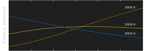
Black-body radiation is the type of electromagnetic radiation within or surrounding a body in thermodynamic equilibrium with its environment, or emitted by a black body (an opaque and non-reflective body) held at constant, uniform temperature. The radiation has a specific spectrum and intensity that depends only on the temperature of the body.
A black-body at room temperature appears black, as most of the energy it radiates is infra-red and cannot be perceived by the human eye. At higher temperatures, black bodies glow with increasing intensity and colors that range from dull red to blindingly brilliant blue-white as the temperature increases.
The Black Body Ultraviolet Catastrophe Experiment
In photography, color temperature describes the spectrum of light which is radiated from a “blackbody” with that surface temperature. A blackbody is an object which absorbs all incident light — neither reflecting it nor allowing it to pass through.
The Sun closely approximates a black-body radiator. Another rough analogue of blackbody radiation in our day to day experience might be in heating a metal or stone: these are said to become “red hot” when they attain one temperature, and then “white hot” for even higher temperatures. Similarly, black bodies at different temperatures also have varying color temperatures of “white light.”
Despite its name, light which may appear white does not necessarily contain an even distribution of colors across the visible spectrum.
Although planets and stars are neither in thermal equilibrium with their surroundings nor perfect black bodies, black-body radiation is used as a first approximation for the energy they emit. Black holes are near-perfect black bodies, and it is believed that they emit black-body radiation (called Hawking radiation), with a temperature that depends on the mass of the hole.
1 to 100% Stepless Dimming, 1500 Lux Brightness at 3.3′
LCD Info Screen. Powered by an L-series battery, D-Tap, or USB-C
Because the light has a variable color range of 3200 to 9500K, when the light is set to 5500K (daylight balanced) both sets of LEDs are on at full, providing the maximum brightness from this fixture when compared to using the light at 3200 or 9500K.
The LCD screen provides information on the fixture’s output as well as the charge state of the battery. The screen also indicates whether the adjustment knob is controlling brightness or color temperature. To switch from brightness to CCT or CCT to brightness, just apply a short press to the adjustment knob.
The included cold shoe ball joint adapter enables mounting the light to your camera’s accessory shoe via the 1/4″-20 threaded hole on the fixture. In addition, the bottom of the cold shoe foot features a 3/8″-16 threaded hole, and includes a 3/8″-16 to 1/4″-20 reducing bushing.
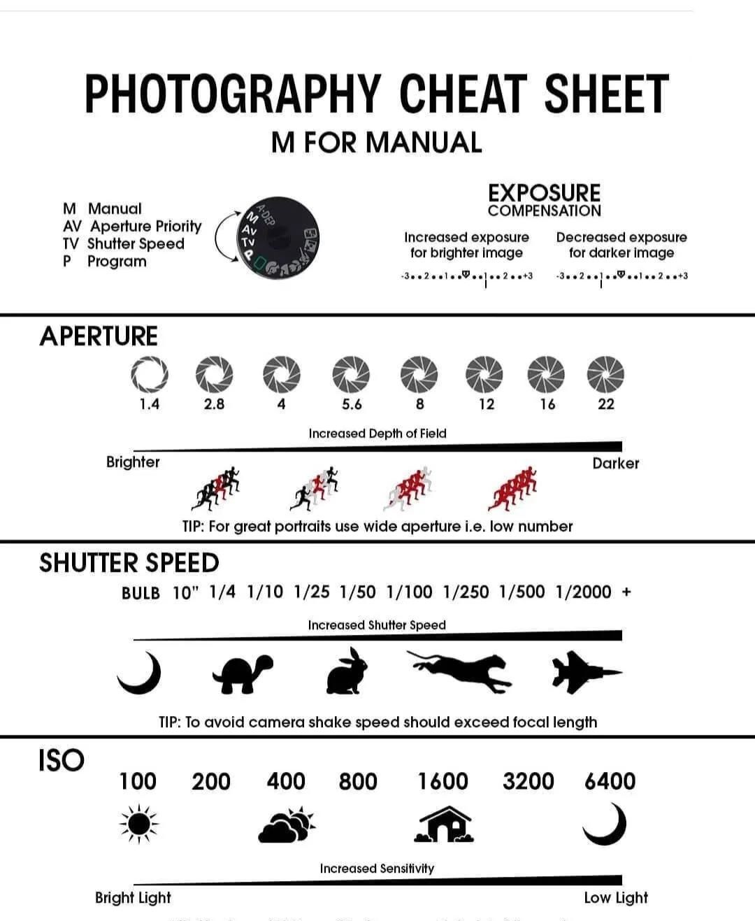
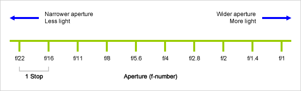
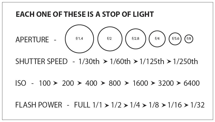
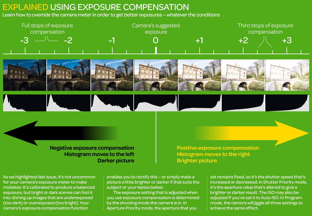
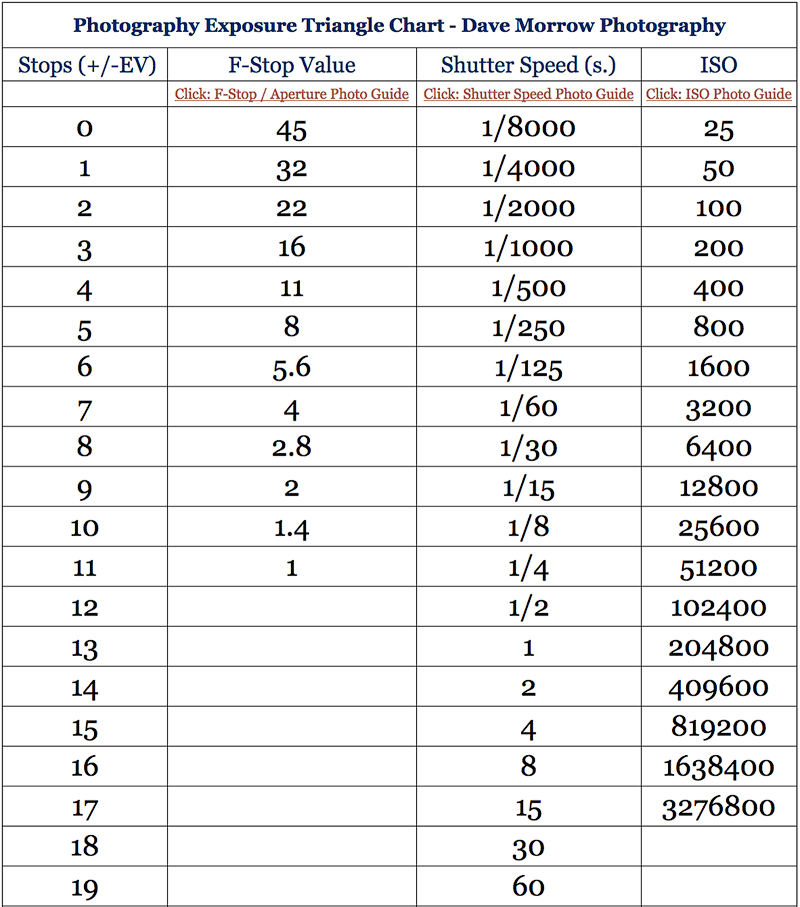
An exposure stop is a unit measurement of Exposure as such it provides a universal linear scale to measure the increase and decrease in light, exposed to the image sensor, due to changes in shutter speed, iso and f-stop.
+-1 stop is a doubling or halving of the amount of light let in when taking a photo
1 EV (exposure value) is just another way to say one stop of exposure change.
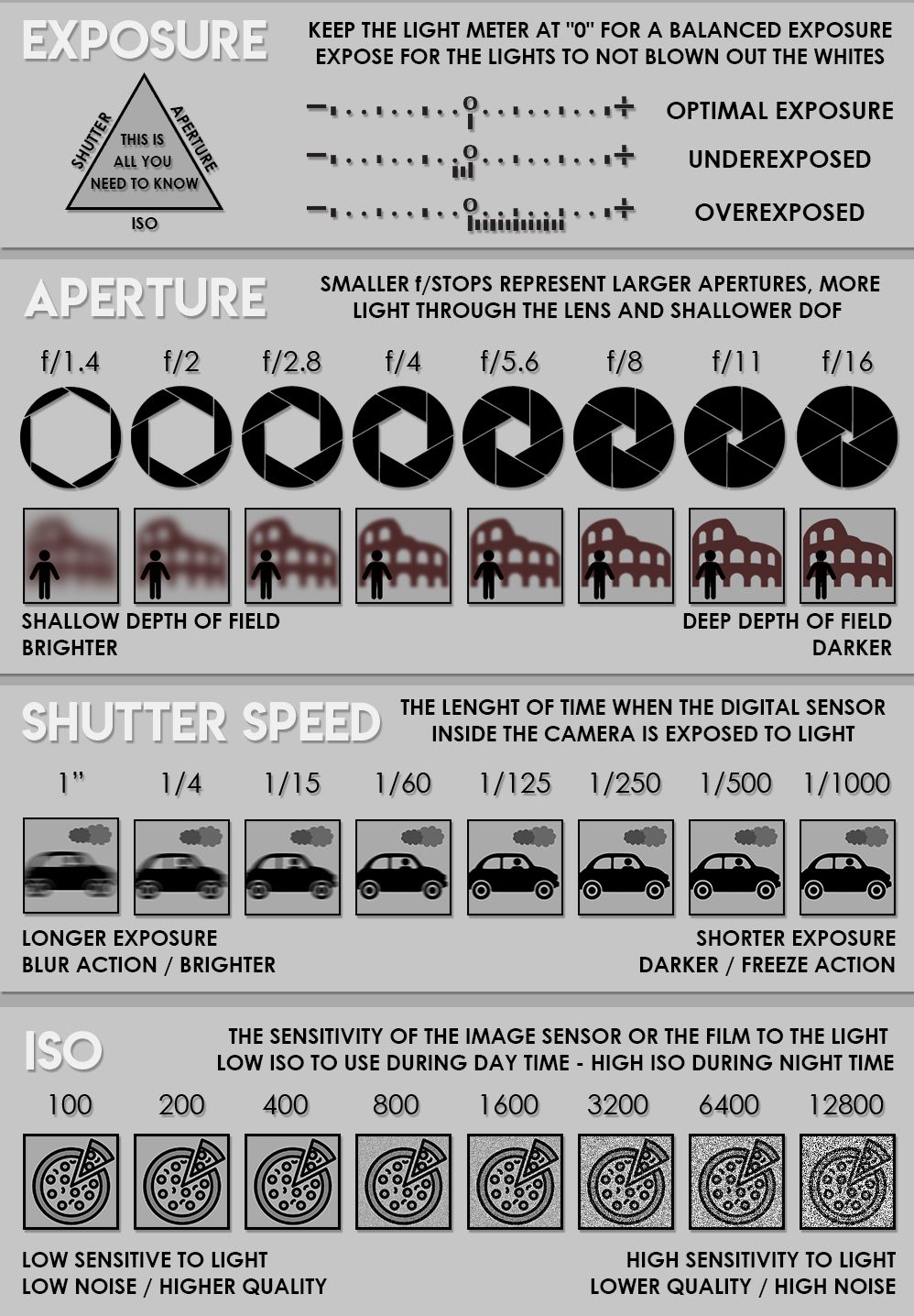
Same applies to shutter speed, iso and aperture.
Doubling or halving your shutter speed produces an increase or decrease of 1 stop of exposure.
Doubling or halving your iso speed produces an increase or decrease of 1 stop of exposure.
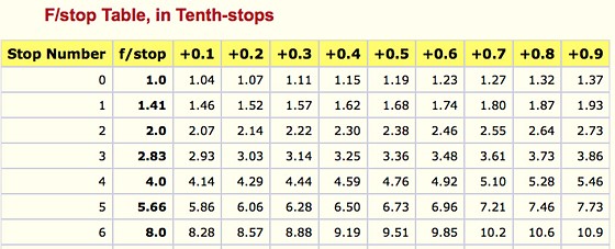
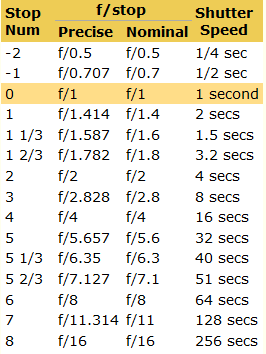
Because of the way f-stop numbers are calculated (ratio of focal length/lens diameter, where focal length is the distance between the lens and the sensor), an f-stop doesn’t relate to a doubling or halving of the value, but to the doubling/halving of the area coverage of a lens in relation to its focal length. And as such, to a multiplying or dividing by 1.41 (the square root of 2). For example, going from f/2.8 to f/4 is a decrease of 1 stop because 4 = 2.8 * 1.41. Changing from f/16 to f/11 is an increase of 1 stop because 11 = 16 / 1.41.
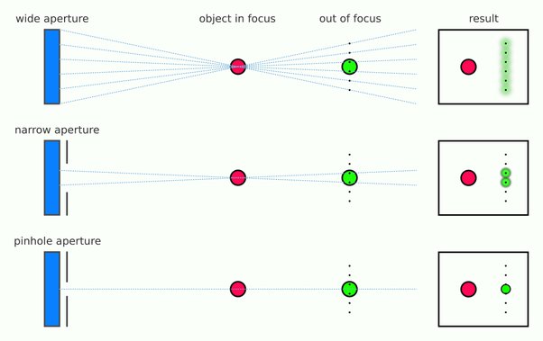
A wider aperture means that light proceeding from the foreground, subject, and background is entering at more oblique angles than the light entering less obliquely.
Consider that absolutely everything is bathed in light, therefore light bouncing off of anything is effectively omnidirectional. Your camera happens to be picking up a tiny portion of the light that’s bouncing off into infinity.
Now consider that the wider your iris/aperture, the more of that omnidirectional light you’re picking up:
When you have a very narrow iris you are eliminating a lot of oblique light. Whatever light enters, from whatever distance, enters moderately parallel as a whole. When you have a wide aperture, much more light is entering at a multitude of angles. Your lens can only focus the light from one depth – the foreground/background appear blurred because it cannot be focused on.
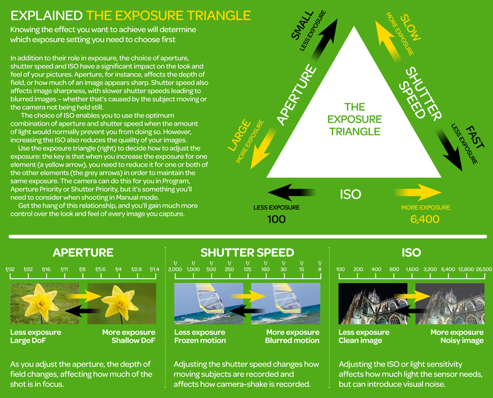
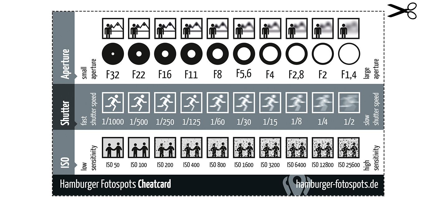
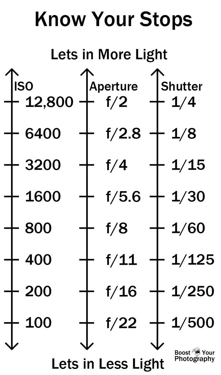
The great thing about stops is that they give us a way to directly compare shutter speed, aperture diameter, and ISO speed. This means that we can easily swap these three components about while keeping the overall exposure the same.
Note. All three of these measurements (aperture, shutter, iso) have full stops, half stops and third stops, but if you look at the numbers they aren’t always consistent. For example, a one third stop between ISO100 and ISO 200 would be ISO133, yet most cameras are marked at ISO125.
Third-stops are especially important as they’re the increment that most cameras use for their settings. These are just imaginary divisions in each stop.
From a practical standpoint manufacturers only standardize the full stops, meaning that while they try and stay somewhat consistent there is some rounding up going on between the smaller numbers.
“a simple yet effective technique to estimate lighting in a single input image. Current techniques rely heavily on HDR panorama datasets to train neural networks to regress an input with limited field-of-view to a full environment map. However, these approaches often struggle with real-world, uncontrolled settings due to the limited diversity and size of their datasets. To address this problem, we leverage diffusion models trained on billions of standard images to render a chrome ball into the input image. Despite its simplicity, this task remains challenging: the diffusion models often insert incorrect or inconsistent objects and cannot readily generate images in HDR format. Our research uncovers a surprising relationship between the appearance of chrome balls and the initial diffusion noise map, which we utilize to consistently generate high-quality chrome balls. We further fine-tune an LDR difusion model (Stable Diffusion XL) with LoRA, enabling it to perform exposure bracketing for HDR light estimation. Our method produces convincing light estimates across diverse settings and demonstrates superior generalization to in-the-wild scenarios.”
DISCLAIMER – Links and images on this website may be protected by the respective owners’ copyright. All data submitted by users through this site shall be treated as freely available to share.


![[gamma correction test]](http://www.madore.org/~david/misc/color/gammatest.png "sRGB gamma correction test")