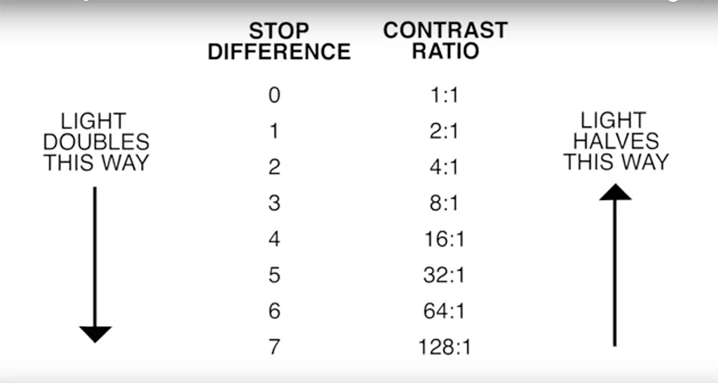
To measure the contrast ratio you will need a light meter. The process starts with you measuring the main source of light, or the key light.
Get a reading from the brightest area on the face of your subject. Then, measure the area lit by the secondary light, or fill light. To make sense of what you have just measured you have to understand that the information you have just gathered is in F-stops, a measure of light. With each additional F-stop, for example going one stop from f/1.4 to f/2.0, you create a doubling of light. The reverse is also true; moving one stop from f/8.0 to f/5.6 results in a halving of the light.
Let’s say you grabbed a measurement from your key light of f/8.0. Then, when you measured your fill light area, you get a reading of f/4.0. This will lead you to a contrast ratio of 4:1 because there are two stops between f/4.0 and f/8.0 and each stop doubles the amount of light. In other words, two stops x twice the light per stop = four times as much light at f/8.0 than at f/4.0.
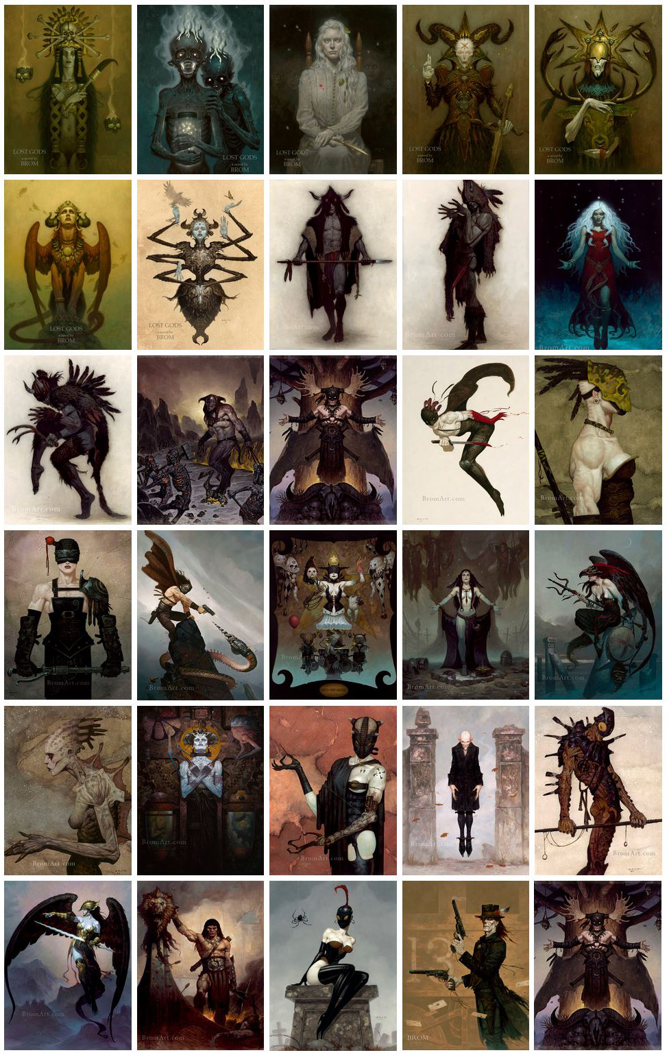
Hand drawn sketch | Models made in CC4 with ZBrush | Textures in Substance Painter | Paint over in Photoshop | Renders, Animation, VFX with AI. Each 5-8 hours spread over a couple days.
As I continue to explore the use of AI tools to enhance my 3D character creation process, I discover they can be incredibly useful during the previsualization phase to see what a character might ultimately look like in production. I selectively use AI to enhance and accelerate my creative process, not to replace it or use it as an end to end solution.
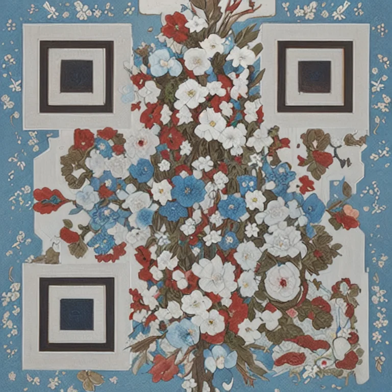
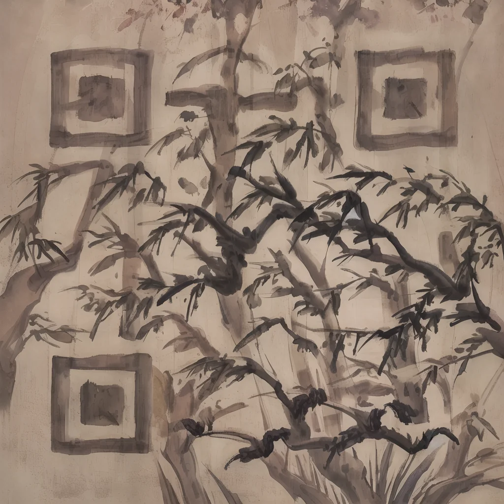
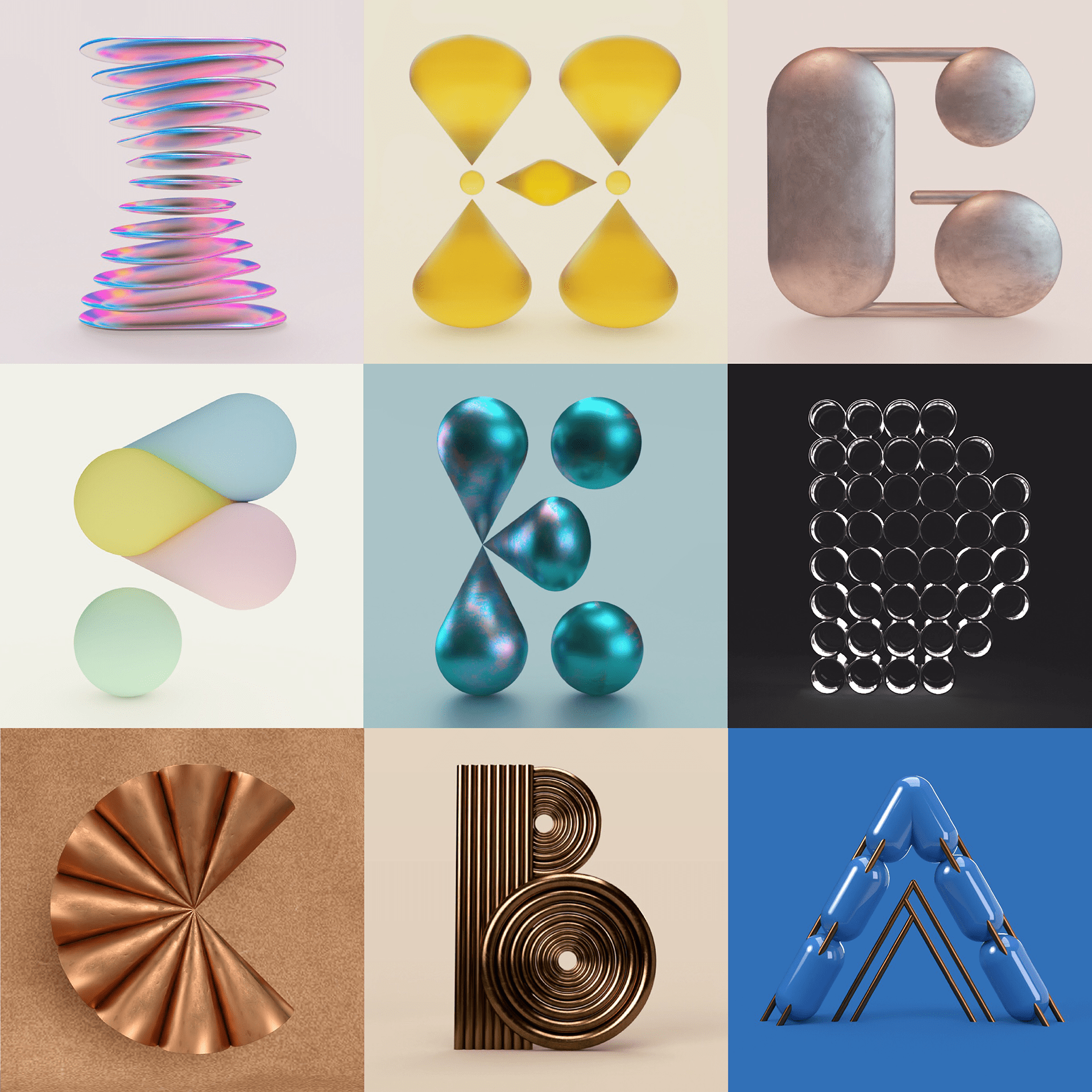
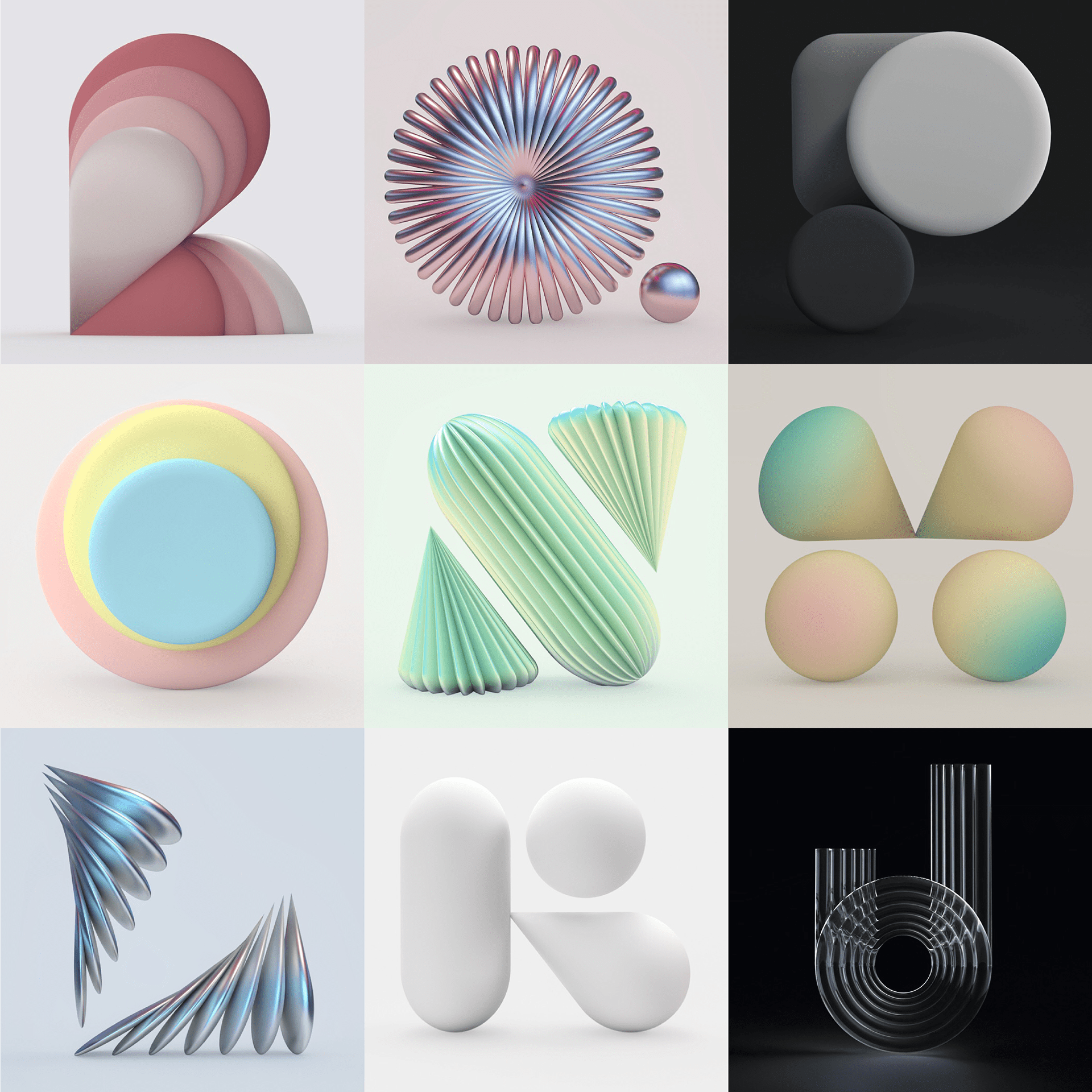
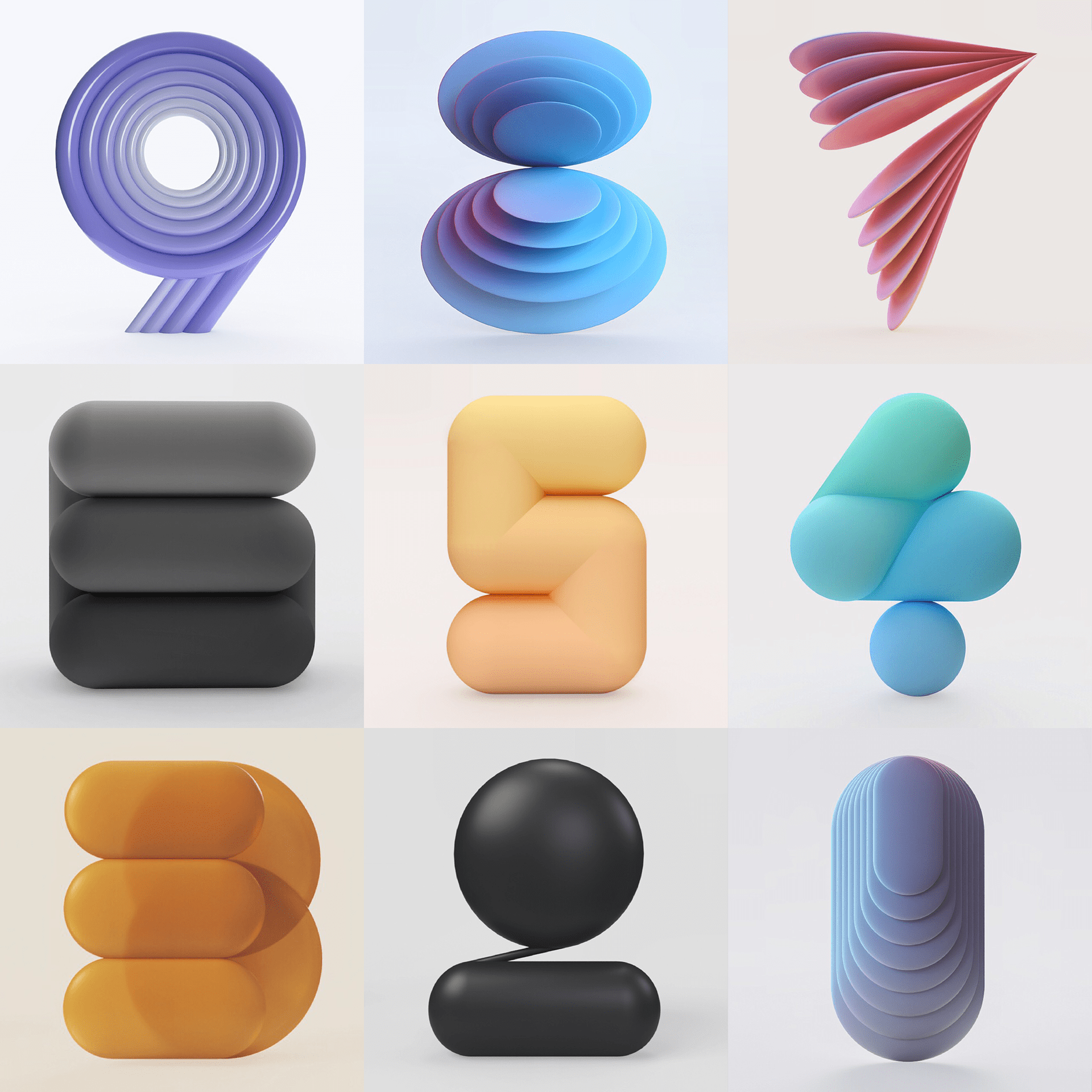
Every Project I work on I always create a stylization Cheat sheet. Every project is unique but some principles carry over no matter what. This is a sheet I use a lot when I work on isometric stylized projects to help keep my assets consistent and interesting. None of these concepts are my own, just lots of tips I learned over the years. I have also added this to a page on my website, will continue to update with more tips and tricks, just need time to compile it all :)
In the retina, photoreceptors, bipolar cells, and horizontal cells work together to process visual information before it reaches the brain. Here’s how each cell type contributes to vision:
1. Photoreceptors
Types: There are two main types of photoreceptors: rods and cones.
Rods: Specialized for low-light and peripheral vision; they help us see in dim lighting and detect motion.
Cones: Specialized for color and detail; they function best in bright light and are concentrated in the central retina (the fovea), allowing for high-resolution vision.
Function: Photoreceptors convert light into electrical signals. When light hits the retina, photoreceptors undergo a chemical change, triggering an electrical response that initiates the visual process. Rods and cones detect different intensities and colors, providing the foundation for brightness and color perception.
2. Bipolar Cells
Function: Bipolar cells act as intermediaries, connecting photoreceptors to ganglion cells, which send signals to the brain. They receive input from photoreceptors and relay it to the retinal ganglion cells.
On and Off Bipolar Cells: Some bipolar cells are ON cells, responding when light is detected (depolarizing in light), and others are OFF cells, responding in darkness (depolarizing in the absence of light). This division allows for more precise contrast detection and the ability to distinguish light from dark areas in the visual field.
3. Horizontal Cells
Function: Horizontal cells connect photoreceptors to each other and create lateral interactions between them. They integrate signals from multiple photoreceptors, allowing them to adjust the sensitivity of neighboring photoreceptors in response to varying light conditions.
Lateral Inhibition: This process improves visual contrast and sharpness by making the borders between light and dark areas more distinct, enhancing our ability to perceive edges and fine detail.
These three types of cells work together to help the retina preprocess visual information and perception, emphasizing contrast and adjusting for different lighting conditions before signals are sent to the brain for further processing and interpretation.
RGBW (RGB + White) LED strip uses a 4-in-1 LED chip made up of red, green, blue, and white.
RGBWW (RGB + White + Warm White) LED strip uses either a 5-in-1 LED chip with red, green, blue, white, and warm white for color mixing. The only difference between RGBW and RGBWW is the intensity of the white color. The term RGBCCT consists of RGB and CCT. CCT (Correlated Color Temperature) means that the color temperature of the led strip light can be adjusted to change between warm white and white. Thus, RGBWW strip light is another name of RGBCCT strip.
RGBCW is the acronym for Red, Green, Blue, Cold, and Warm. These 5-in-1 chips are used in supper bright smart LED lighting products
“a simple yet effective technique to estimate lighting in a single input image. Current techniques rely heavily on HDR panorama datasets to train neural networks to regress an input with limited field-of-view to a full environment map. However, these approaches often struggle with real-world, uncontrolled settings due to the limited diversity and size of their datasets. To address this problem, we leverage diffusion models trained on billions of standard images to render a chrome ball into the input image. Despite its simplicity, this task remains challenging: the diffusion models often insert incorrect or inconsistent objects and cannot readily generate images in HDR format. Our research uncovers a surprising relationship between the appearance of chrome balls and the initial diffusion noise map, which we utilize to consistently generate high-quality chrome balls. We further fine-tune an LDR difusion model (Stable Diffusion XL) with LoRA, enabling it to perform exposure bracketing for HDR light estimation. Our method produces convincing light estimates across diverse settings and demonstrates superior generalization to in-the-wild scenarios.”
Note. The Median Cut algorithm is typically used for color quantization, which involves reducing the number of colors in an image while preserving its visual quality. It doesn’t directly provide a way to identify the brightest areas in an image. However, if you’re interested in identifying the brightest areas, you might want to look into other methods like thresholding, histogram analysis, or edge detection, through openCV for example.
Here is an openCV example:
# bottom left coordinates = 0,0
import numpy as np
import cv2

# Load the HDR or EXR image
image = cv2.imread('your_image_path.exr', cv2.IMREAD_UNCHANGED)  # Load as-is without modification

# Calculate the luminance from the HDR channels (assuming RGB format)
luminance = np.dot(image[..., :3], [0.299, 0.587, 0.114])

# Set a threshold value based on estimated EV
threshold_value = 2.4  # Estimated threshold value based on 4.8 EV

# Apply the threshold to identify bright areas
# The luminance array contains the calculated luminance values for each pixel in the image. # The threshold_value is a user-defined value that represents a cutoff point, separating "bright" and "dark" areas in terms of perceived luminance.
thresholded = (luminance > threshold_value) * 255

# Convert the thresholded image to uint8 for contour detection
thresholded = thresholded.astype(np.uint8)

# Find contours of the bright areas
contours, _ = cv2.findContours(thresholded, cv2.RETR_EXTERNAL, cv2.CHAIN_APPROX_SIMPLE)

# Create a list to store the bounding boxes of bright areas
bright_areas = []

# Iterate through contours and extract bounding boxes for contour in contours:
x, y, w, h = cv2.boundingRect(contour)

# Adjust y-coordinate based on bottom-left origin
y_bottom_left_origin = image.shape[0] - (y + h) bright_areas.append((x, y_bottom_left_origin, x + w, y_bottom_left_origin + h))

# Store as (x1, y1, x2, y2)
# Print the identified bright areas
print("Bright Areas (x1, y1, x2, y2):") for area in bright_areas: print(area)
More details
Luminance and Exposure in an EXR Image:
An EXR (Extended Dynamic Range) image format is often used to store high dynamic range (HDR) images that contain a wide range of luminance values, capturing both dark and bright areas.
Luminance refers to the perceived brightness of a pixel in an image. In an RGB image, luminance is often calculated using a weighted sum of the red, green, and blue channels, where different weights are assigned to each channel to account for human perception.
In an EXR image, the pixel values can represent radiometrically accurate scene values, including actual radiance or irradiance levels. These values are directly related to the amount of light emitted or reflected by objects in the scene.
The luminance line is calculating the luminance of each pixel in the image using a weighted sum of the red, green, and blue channels. The three float values [0.299, 0.587, 0.114] are the weights used to perform this calculation.
These weights are based on the concept of luminosity, which aims to approximate the perceived brightness of a color by taking into account the human eye’s sensitivity to different colors. The values are often derived from the NTSC (National Television System Committee) standard, which is used in various color image processing operations.
Here’s the breakdown of the float values:
0.299: Weight for the red channel.
0.587: Weight for the green channel.
0.114: Weight for the blue channel.
The weighted sum of these channels helps create a grayscale image where the pixel values represent the perceived brightness. This technique is often used when converting a color image to grayscale or when calculating luminance for certain operations, as it takes into account the human eye’s sensitivity to different colors.
For the threshold, remember that the exact relationship between EV values and pixel values can depend on the tone-mapping or normalization applied to the HDR image, as well as the dynamic range of the image itself.
To establish a relationship between exposure and the threshold value, you can consider the relationship between linear and logarithmic scales:
Linear and Logarithmic Scales:
Exposure values in an EXR image are often represented in logarithmic scales, such as EV (exposure value). Each increment in EV represents a doubling or halving of the amount of light captured.
Threshold values for luminance thresholding are usually linear, representing an actual luminance level.
Conversion Between Scales:
To establish a mathematical relationship, you need to convert between the logarithmic exposure scale and the linear threshold scale.
One common method is to use a power function. For instance, you can use a power function to convert EV to a linear intensity value.
threshold_value = base_value * (2 ** EV)
Here, EV is the exposure value, base_value is a scaling factor that determines the relationship between EV and threshold_value, and 2 ** EV is used to convert the logarithmic EV to a linear intensity value.
Choosing the Base Value:
The base_value factor should be determined based on the dynamic range of your EXR image and the specific luminance values you are dealing with.
You may need to experiment with different values of base_value to achieve the desired separation of bright areas from the rest of the image.
Let’s say you have an EXR image with a dynamic range of 12 EV, which is a common range for many high dynamic range images. In this case, you want to set a threshold value that corresponds to a certain number of EV above the middle gray level (which is often considered to be around 0.18).
Here’s an example of how you might determine a base_value to achieve this:
# Define the dynamic range of the image in EV
dynamic_range = 12

# Choose the desired number of EV above middle gray for thresholding
desired_ev_above_middle_gray = 2

# Calculate the threshold value based on the desired EV above middle gray
threshold_value = 0.18 * (2 ** (desired_ev_above_middle_gray / dynamic_range))

print("Threshold Value:", threshold_value)
A way to approximate complex lighting in ultra realistic renders.
All SH lighting techniques involve replacing parts of standard lighting equations with spherical functions that have been projected into frequency space using the spherical harmonics as a basis.
DISCLAIMER – Links and images on this website may be protected by the respective owners’ copyright. All data submitted by users through this site shall be treated as freely available to share.