


COMPOSITION
-
Photography basics: Depth of Field and composition
Read more: Photography basics: Depth of Field and compositionDepth of field is the range within which focusing is resolved in a photo.
Aperture has a huge affect on to the depth of field.
Changing the f-stops (f/#) of a lens will change aperture and as such the DOF.
f-stops are a just certain number which is telling you the size of the aperture. That’s how f-stop is related to aperture (and DOF).
If you increase f-stops, it will increase DOF, the area in focus (and decrease the aperture). On the other hand, decreasing the f-stop it will decrease DOF (and increase the aperture).
The red cone in the figure is an angular representation of the resolution of the system. Versus the dotted lines, which indicate the aperture coverage. Where the lines of the two cones intersect defines the total range of the depth of field.
This image explains why the longer the depth of field, the greater the range of clarity.

-
Composition and The Expressive Nature Of Light
Read more: Composition and The Expressive Nature Of Lighthttp://www.huffingtonpost.com/bill-danskin/post_12457_b_10777222.html
George Sand once said “ The artist vocation is to send light into the human heart.”


DESIGN


COLOR
-
Tim Kang – calibrated white light values in sRGB color space
Read more: Tim Kang – calibrated white light values in sRGB color space8bit sRGB encoded
2000K 255 139 22
2700K 255 172 89
3000K 255 184 109
3200K 255 190 122
4000K 255 211 165
4300K 255 219 178
D50 255 235 205
D55 255 243 224
D5600 255 244 227
D6000 255 249 240
D65 255 255 255
D10000 202 221 255
D20000 166 196 2558bit Rec709 Gamma 2.4
2000K 255 145 34
2700K 255 177 97
3000K 255 187 117
3200K 255 193 129
4000K 255 214 170
4300K 255 221 182
D50 255 236 208
D55 255 243 226
D5600 255 245 229
D6000 255 250 241
D65 255 255 255
D10000 204 222 255
D20000 170 199 2558bit Display P3 encoded
2000K 255 154 63
2700K 255 185 109
3000K 255 195 127
3200K 255 201 138
4000K 255 219 176
4300K 255 225 187
D50 255 239 212
D55 255 245 228
D5600 255 246 231
D6000 255 251 242
D65 255 255 255
D10000 208 223 255
D20000 175 199 25510bit Rec2020 PQ (100 nits)
2000K 520 435 273
2700K 520 466 358
3000K 520 475 384
3200K 520 480 399
4000K 520 495 446
4300K 520 500 458
D50 520 510 482
D55 520 514 497
D5600 520 514 500
D6000 520 517 509
D65 520 520 520
D10000 479 489 520
D20000 448 464 520
-
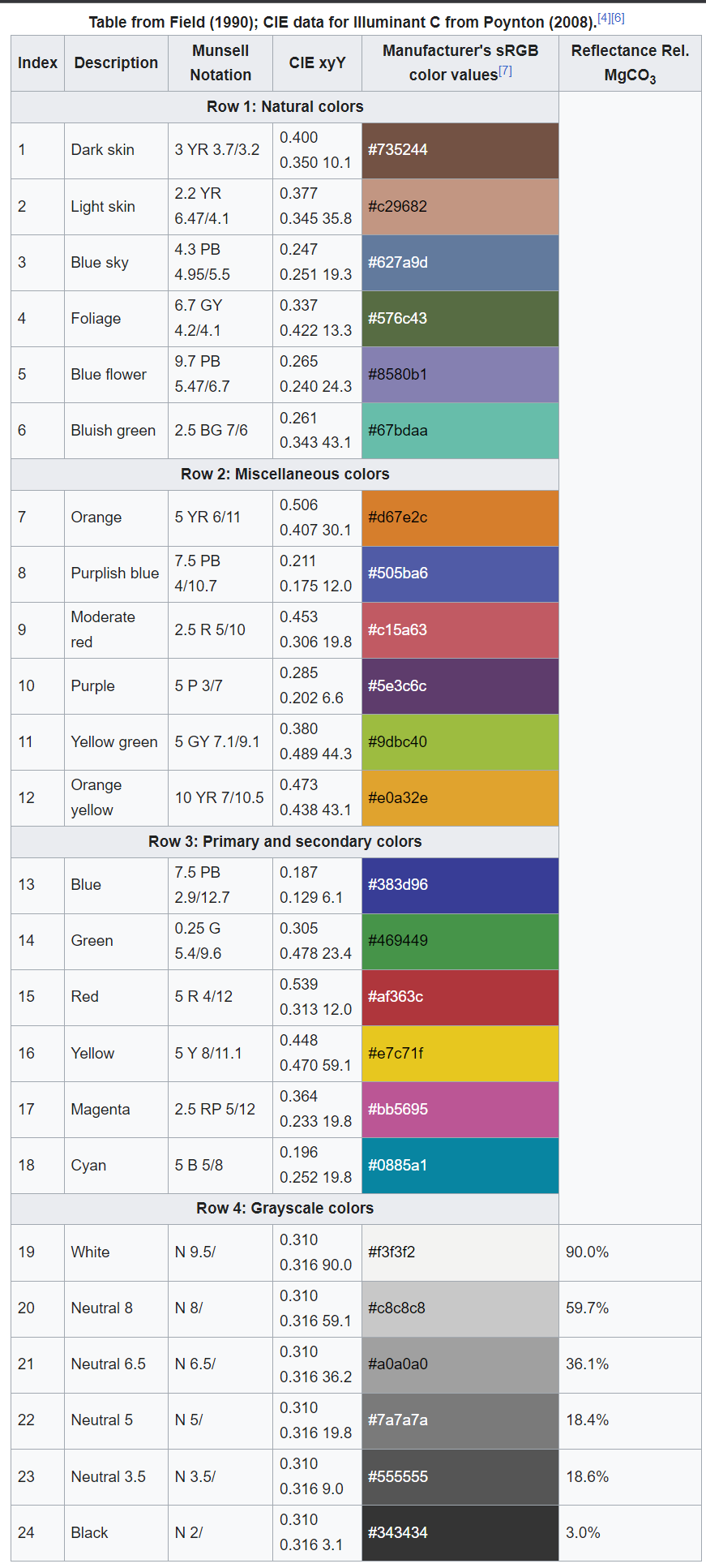
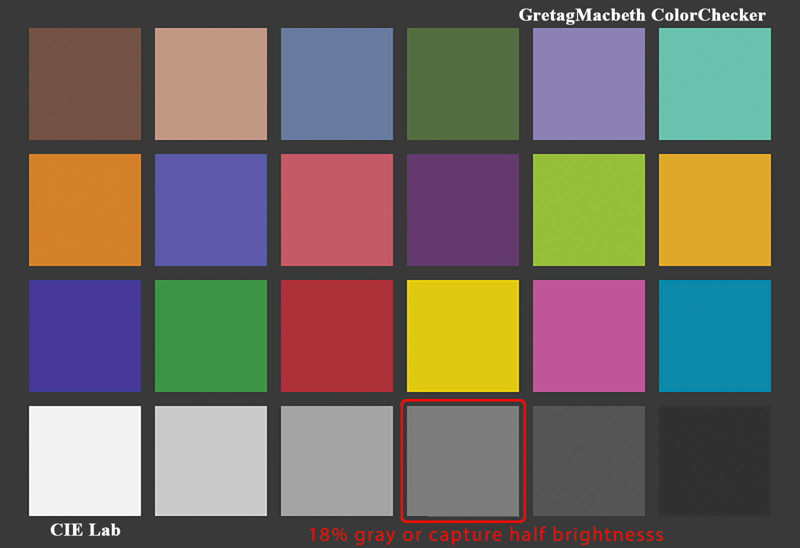
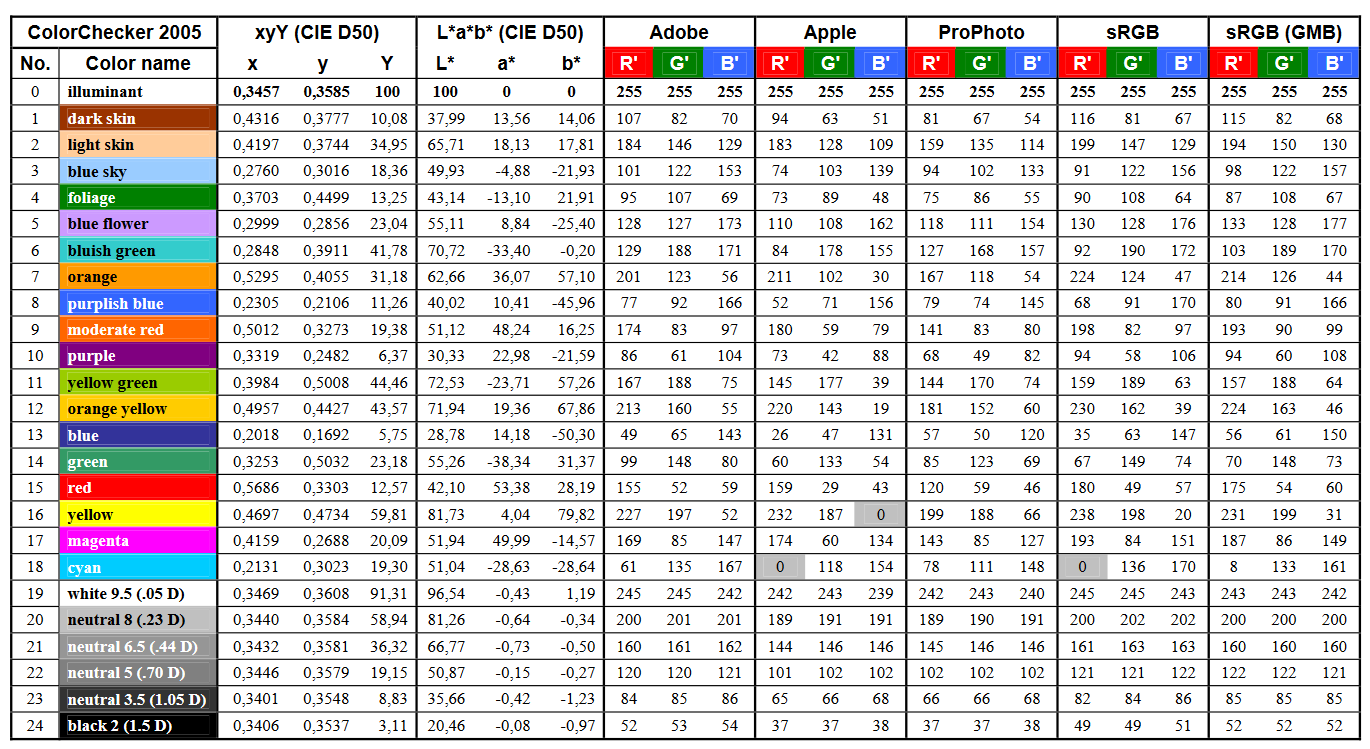
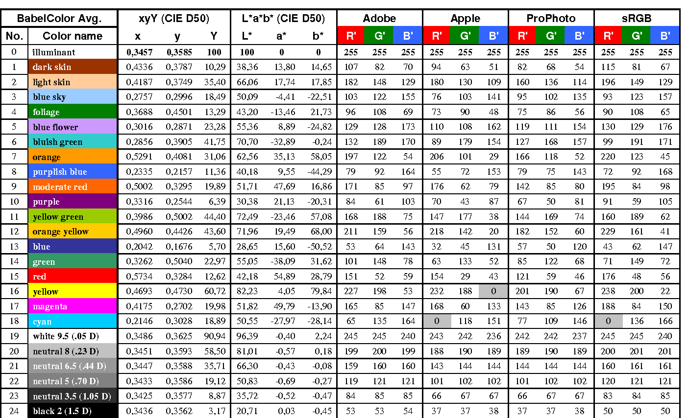
GretagMacbeth Color Checker Numeric Values and Middle Gray
Read more: GretagMacbeth Color Checker Numeric Values and Middle GrayThe human eye perceives half scene brightness not as the linear 50% of the present energy (linear nature values) but as 18% of the overall brightness. We are biased to perceive more information in the dark and contrast areas. A Macbeth chart helps with calibrating back into a photographic capture into this “human perspective” of the world.
https://en.wikipedia.org/wiki/Middle_gray
In photography, painting, and other visual arts, middle gray or middle grey is a tone that is perceptually about halfway between black and white on a lightness scale in photography and printing, it is typically defined as 18% reflectance in visible light
Light meters, cameras, and pictures are often calibrated using an 18% gray card[4][5][6] or a color reference card such as a ColorChecker. On the assumption that 18% is similar to the average reflectance of a scene, a grey card can be used to estimate the required exposure of the film.
https://en.wikipedia.org/wiki/ColorChecker
The exposure meter in the camera does not know whether the subject itself is bright or not. It simply measures the amount of light that comes in, and makes a guess based on that. The camera will aim for 18% gray independently, meaning if you take a photo of an entirely white surface, and an entirely black surface you should get two identical images which both are gray (at least in theory). Thus enters the Macbeth chart.
<!–more–>
Note that Chroma Key Green is reasonably close to an 18% gray reflectance.
http://www.rags-int-inc.com/PhotoTechStuff/MacbethTarget/

No Camera Data 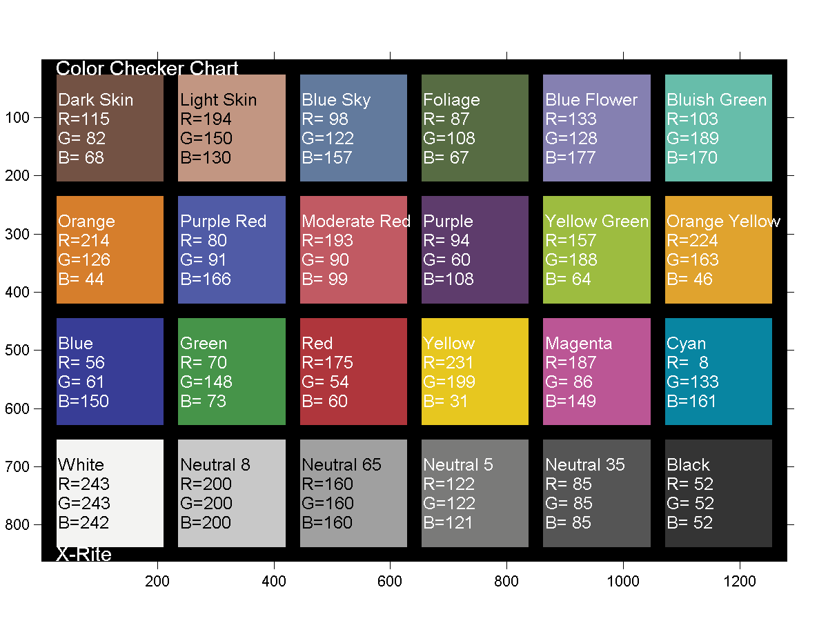
https://upload.wikimedia.org/wikipedia/commons/b/b4/CIE1931xy_ColorChecker_SMIL.svg

RGB coordinates of the Macbeth ColorChecker
https://pdfs.semanticscholar.org/0e03/251ad1e6d3c3fb9cb0b1f9754351a959e065.pdf
-
Willem Zwarthoed – Aces gamut in VFX production pdf
Read more: Willem Zwarthoed – Aces gamut in VFX production pdfhttps://www.provideocoalition.com/color-management-part-12-introducing-aces/
Local copy:
https://www.slideshare.net/hpduiker/acescg-a-common-color-encoding-for-visual-effects-applications


LIGHTING
-
studiobinder.com – What is Tenebrism and Hard Lighting — The Art of Light and Shadow and chiaroscuro Explained
Read more: studiobinder.com – What is Tenebrism and Hard Lighting — The Art of Light and Shadow and chiaroscuro Explainedhttps://www.studiobinder.com/blog/what-is-tenebrism-art-definition/
https://www.studiobinder.com/blog/what-is-hard-light-photography/


-
Neural Microfacet Fields for Inverse Rendering
Read more: Neural Microfacet Fields for Inverse Renderinghttps://half-potato.gitlab.io/posts/nmf/

-
Photography basics: Why Use a (MacBeth) Color Chart?
Read more: Photography basics: Why Use a (MacBeth) Color Chart?Start here: https://www.pixelsham.com/2013/05/09/gretagmacbeth-color-checker-numeric-values/
https://www.studiobinder.com/blog/what-is-a-color-checker-tool/


In LightRoom

in Final Cut

in Nuke
Note: In Foundry’s Nuke, the software will map 18% gray to whatever your center f/stop is set to in the viewer settings (f/8 by default… change that to EV by following the instructions below).
You can experiment with this by attaching an Exposure node to a Constant set to 0.18, setting your viewer read-out to Spotmeter, and adjusting the stops in the node up and down. You will see that a full stop up or down will give you the respective next value on the aperture scale (f8, f11, f16 etc.).One stop doubles or halves the amount or light that hits the filmback/ccd, so everything works in powers of 2.
So starting with 0.18 in your constant, you will see that raising it by a stop will give you .36 as a floating point number (in linear space), while your f/stop will be f/11 and so on.If you set your center stop to 0 (see below) you will get a relative readout in EVs, where EV 0 again equals 18% constant gray.

In other words. Setting the center f-stop to 0 means that in a neutral plate, the middle gray in the macbeth chart will equal to exposure value 0. EV 0 corresponds to an exposure time of 1 sec and an aperture of f/1.0.
This will set the sun usually around EV12-17 and the sky EV1-4 , depending on cloud coverage.
To switch Foundry’s Nuke’s SpotMeter to return the EV of an image, click on the main viewport, and then press s, this opens the viewer’s properties. Now set the center f-stop to 0 in there. And the SpotMeter in the viewport will change from aperture and fstops to EV.
-
Key/Fill ratios and scene composition using false colors
Read more: Key/Fill ratios and scene composition using false colors
To measure the contrast ratio you will need a light meter. The process starts with you measuring the main source of light, or the key light.
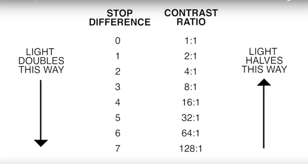
Get a reading from the brightest area on the face of your subject. Then, measure the area lit by the secondary light, or fill light. To make sense of what you have just measured you have to understand that the information you have just gathered is in F-stops, a measure of light. With each additional F-stop, for example going one stop from f/1.4 to f/2.0, you create a doubling of light. The reverse is also true; moving one stop from f/8.0 to f/5.6 results in a halving of the light.
Let’s say you grabbed a measurement from your key light of f/8.0. Then, when you measured your fill light area, you get a reading of f/4.0. This will lead you to a contrast ratio of 4:1 because there are two stops between f/4.0 and f/8.0 and each stop doubles the amount of light. In other words, two stops x twice the light per stop = four times as much light at f/8.0 than at f/4.0.

theslantedlens.com/2017/lighting-ratios-photo-video/
Examples in the post


COLLECTIONS
| Featured AI
| Design And Composition
| Explore posts
POPULAR SEARCHES
unreal | pipeline | virtual production | free | learn | photoshop | 360 | macro | google | nvidia | resolution | open source | hdri | real-time | photography basics | nuke
FEATURED POSTS
-
Free fonts
-
Photography basics: Shutter angle and shutter speed and motion blur
-
Convert 2D Images or Text to 3D Models
-
Methods for creating motion blur in Stop motion
-
Most common ways to smooth 3D prints
-
copypastecharacter.com – alphabets, special characters, alt codes and symbols library
-
Glossary of Lighting Terms – cheat sheet
-
Generative AI Glossary / AI Dictionary / AI Terminology
Social Links
DISCLAIMER – Links and images on this website may be protected by the respective owners’ copyright. All data submitted by users through this site shall be treated as freely available to share.
