Deepfake technology is a type of artificial intelligence used to create convincing fake images, videos and audio recordings. The term describes both the technology and the resulting bogus content and is a portmanteau of deep learning and fake.
Deepfakes often transform existing source content where one person is swapped for another. They also create entirely original content where someone is represented doing or saying something they didn’t do or say.
Deepfakes aren’t edited or photoshopped videos or images. In fact, they’re created using specialized algorithms that blend existing and new footage. For example, subtle facial features of people in images are analyzed through machine learning (ML) to manipulate them within the context of other videos.
Deepfakes uses two algorithms — a generator and a discriminator — to create and refine fake content. The generator builds a training data set based on the desired output, creating the initial fake digital content, while the discriminator analyzes how realistic or fake the initial version of the content is. This process is repeated, enabling the generator to improve at creating realistic content and the discriminator to become more skilled at spotting flaws for the generator to correct.
The combination of the generator and discriminator algorithms creates a generative adversarial network.
A GANuses deep learning to recognize patterns in real images and then uses those patterns to create the fakes.
When creating a deepfake photograph, a GAN system views photographs of the target from an array of angles to capture all the details and perspectives. When creating a deepfake video, the GAN views the video from various angles and analyzes behavior, movement and speech patterns. This information is then run through the discriminator multiple times to fine-tune the realism of the final image or video.
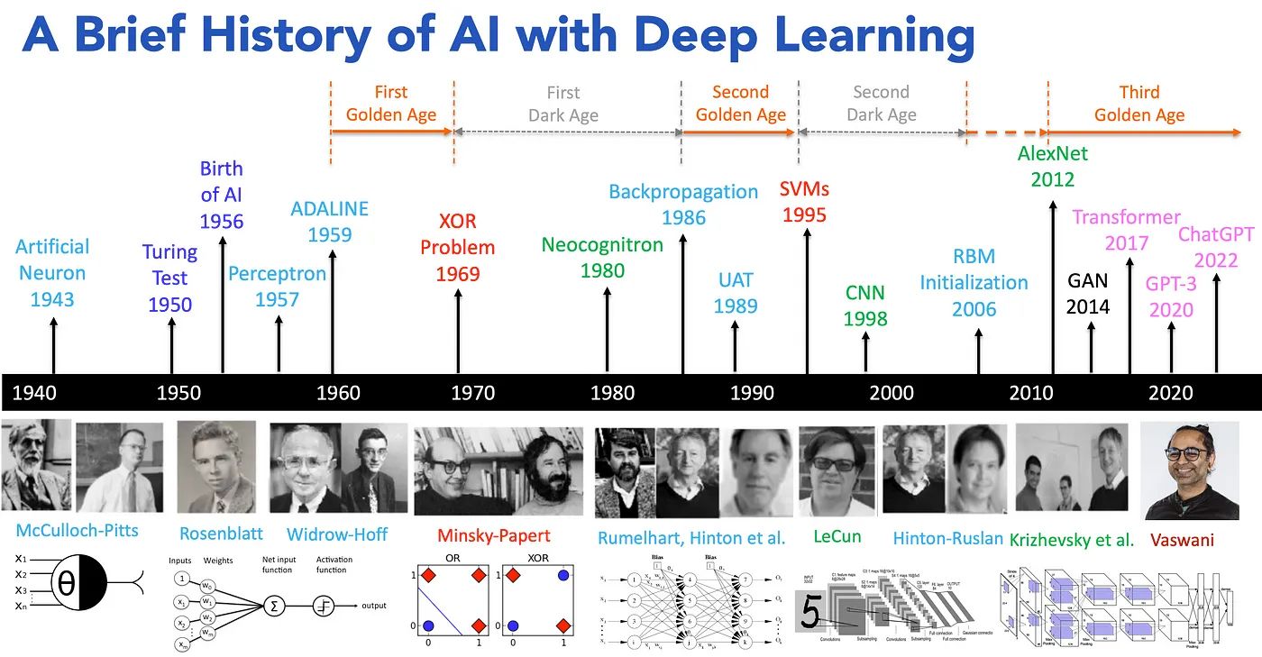
🔹 1943: 𝗠𝗰𝗖𝘂𝗹𝗹𝗼𝗰𝗵 & 𝗣𝗶𝘁𝘁𝘀 create the first artificial neuron. 🔹 1950: 𝗔𝗹𝗮𝗻 𝗧𝘂𝗿𝗶𝗻𝗴 introduces the Turing Test, forever changing the way we view intelligence. 🔹 1956: 𝗝𝗼𝗵𝗻 𝗠𝗰𝗖𝗮𝗿𝘁𝗵𝘆 coins the term “Artificial Intelligence,” marking the official birth of the field. 🔹 1957: 𝗙𝗿𝗮𝗻𝗸 𝗥𝗼𝘀𝗲𝗻𝗯𝗹𝗮𝘁𝘁 invents the Perceptron, one of the first neural networks. 🔹 1959: 𝗕𝗲𝗿𝗻𝗮𝗿𝗱 𝗪𝗶𝗱𝗿𝗼𝘄 and 𝗧𝗲𝗱 𝗛𝗼𝗳𝗳 create ADALINE, a model that would shape neural networks. 🔹 1969: 𝗠𝗶𝗻𝘀𝗸𝘆 & 𝗣𝗮𝗽𝗲𝗿𝘁 solve the XOR problem, but also mark the beginning of the “first AI winter.” 🔹 1980: 𝗞𝘂𝗻𝗶𝗵𝗶𝗸𝗼 𝗙𝘂𝗸𝘂𝘀𝗵𝗶𝗺𝗮 introduces Neocognitron, laying the groundwork for deep learning. 🔹 1986: 𝗚𝗲𝗼𝗳𝗳𝗿𝗲𝘆 𝗛𝗶𝗻𝘁𝗼𝗻 and 𝗗𝗮𝘃𝗶𝗱 𝗥𝘂𝗺𝗲𝗹𝗵𝗮𝗿𝘁 introduce backpropagation, making neural networks viable again. 🔹 1989: 𝗝𝘂𝗱𝗲𝗮 𝗣𝗲𝗮𝗿𝗹 advances UAT (Understanding and Reasoning), building a foundation for AI’s logical abilities. 🔹 1995: 𝗩𝗹𝗮𝗱𝗶𝗺𝗶𝗿 𝗩𝗮𝗽𝗻𝗶𝗸 and 𝗖𝗼𝗿𝗶𝗻𝗻𝗮 𝗖𝗼𝗿𝘁𝗲𝘀 develop Support Vector Machines (SVMs), a breakthrough in machine learning. 🔹 1998: 𝗬𝗮𝗻𝗻 𝗟𝗲𝗖𝘂𝗻 popularizes Convolutional Neural Networks (CNNs), revolutionizing image recognition. 🔹 2006: 𝗚𝗲𝗼𝗳𝗳𝗿𝗲𝘆 𝗛𝗶𝗻𝘁𝗼𝗻 and 𝗥𝘂𝘀𝗹𝗮𝗻 𝗦𝗮𝗹𝗮𝗸𝗵𝘂𝘁𝗱𝗶𝗻𝗼𝘃 introduce deep belief networks, reigniting interest in deep learning. 🔹 2012: 𝗔𝗹𝗲𝘅 𝗞𝗿𝗶𝘇𝗵𝗲𝘃𝘀𝗸𝘆 and 𝗚𝗲𝗼𝗳𝗳𝗿𝗲𝘆 𝗛𝗶𝗻𝘁𝗼𝗻 launch AlexNet, sparking the modern AI revolution in deep learning. 🔹 2014: 𝗜𝗮𝗻 𝗚𝗼𝗼𝗱𝗳𝗲𝗹𝗹𝗼𝘄 introduces Generative Adversarial Networks (GANs), opening new doors for AI creativity. 🔹 2017: 𝗔𝘀𝗵𝗶𝘀𝗵 𝗩𝗮𝘀𝘄𝗮𝗻𝗶 and team introduce Transformers, redefining natural language processing (NLP). 🔹 2020: OpenAI unveils GPT-3, setting a new standard for language models and AI’s capabilities. 🔹 2022: OpenAI releases ChatGPT, democratizing conversational AI and bringing it to the masses.
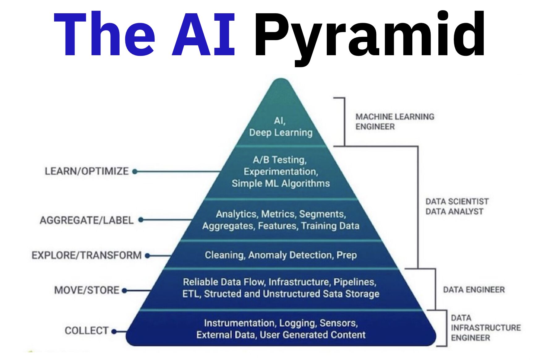
– Collect: Data from sensors, logs, and user input. – Move/Store: Build infrastructure, pipelines, and reliable data flow. – Explore/Transform: Clean, prep, and detect anomalies to make the data usable. – Aggregate/Label: Add analytics, metrics, and labels to create training data. – Learn/Optimize: Experiment, test, and train AI models.
– Instrumentation and logging: Sensors, logs, and external data capture the raw inputs. – Data flow and storage: Pipelines and infrastructure ensure smooth movement and reliable storage. – Exploration and transformation: Data is cleaned, prepped, and anomalies are detected. – Aggregation and labeling: Analytics, metrics, and labels create structured, usable datasets. – Experimenting/AI/ML: Models are trained and optimized using the prepared data. – AI insights and actions: Advanced AI generates predictions, insights, and decisions at the top.
𝗪𝗵𝗼 𝗺𝗮𝗸𝗲𝘀 𝗶𝘁 𝗵𝗮𝗽𝗽𝗲𝗻 𝗮𝗻𝗱 𝗸𝗲𝘆 𝗿𝗼𝗹𝗲𝘀:
– Data Infrastructure Engineers: Build the foundation — collect, move, and store data. – Data Engineers: Prep and transform the data into usable formats. – Data Analysts & Scientists: Aggregate, label, and generate insights. – Machine Learning Engineers: Optimize and deploy AI models.
You’ve been in the VFX Industry for over a decade. Tell us about your journey.
It all started with my older brother giving me a Commodore64 personal computer as a gift back in the late 80′. I realised then I could create something directly from my imagination using this new digital media format. And, eventually, make a living in the process. That led me to start my professional career in 1990. From live TV to games to animation. All the way to live action VFX in the recent years.
I really never stopped to crave to create art since those early days. And I have been incredibly fortunate to work with really great talent along the way, which made my journey so much more effective.
What inspired you to pursue VFX as a career?
An incredible combination of opportunities, really. The opportunity to express myself as an artist and earn money in the process. The opportunity to learn about how the world around us works and how best solve problems. The opportunity to share my time with other talented people with similar passions. The opportunity to grow and adapt to new challenges. The opportunity to develop something that was never done before. A perfect storm of creativity that fed my continuous curiosity about life and genuinely drove my inspiration.
Tell us about the projects you’ve particularly enjoyed working on in your career
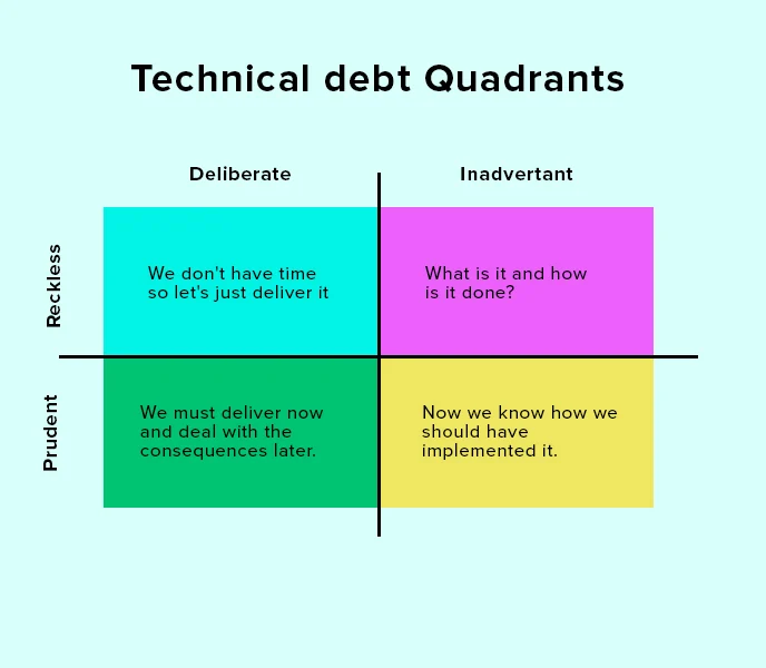
In software development, “technical debt” is a term used to describe the accumulation of shortcuts, suboptimal solutions, and outdated code that occur as developers rush to meet deadlines or prioritize immediate goals over long-term maintainability. While this concept initially seems abstract, its consequences are concrete and can significantly affect the security, usability, and stability of software systems.
The Nature of Technical Debt
Technical debt arises when software engineers choose a less-than-ideal implementation in the interest of saving time or reducing upfront effort. Much like financial debt, these decisions come with an interest rate: over time, the cost of maintaining and updating the system increases, and more effort is required to fix problems that stem from earlier choices. In extreme cases, technical debt can slow development to a crawl, causing future updates or improvements to become far more difficult than they would have been with cleaner, more scalable code.
Impact on Security
One of the most significant threats posed by technical debt is the vulnerability it creates in terms of software security. Outdated code often lacks the latest security patches or is built on legacy systems that are no longer supported. Attackers can exploit these weaknesses, leading to data breaches, ransomware, or other forms of cybercrime. Furthermore, as systems grow more complex and the debt compounds, identifying and fixing vulnerabilities becomes increasingly challenging. Failing to address technical debt leaves an organization exposed to security risks that may only become apparent after a costly incident.
Impact on Usability
Technical debt also affects the user experience. Systems burdened by outdated code often become clunky and slow, leading to poor usability. Engineers may find themselves continuously patching minor issues rather than implementing larger, user-centric improvements. Over time, this results in a product that feels antiquated, is difficult to use, or lacks modern functionality. In a competitive market, poor usability can alienate users, causing a loss of confidence and driving them to alternative products or services.
Impact on Stability
Stability is another critical area impacted by technical debt. As developers add features or make updates to systems weighed down by previous quick fixes, they run the risk of introducing bugs or causing system crashes. The tangled, fragile nature of code laden with technical debt makes troubleshooting difficult and increases the likelihood of cascading failures. Over time, instability in the software can erode both the trust of users and the efficiency of the development team, as more resources are dedicated to resolving recurring issues rather than innovating or expanding the system’s capabilities.
The Long-Term Costs of Ignoring Technical Debt
While technical debt can provide short-term gains by speeding up initial development, the long-term costs are much higher. Unaddressed technical debt can lead to project delays, escalating maintenance costs, and an ever-widening gap between current code and modern best practices. The more technical debt accumulates, the harder and more expensive it becomes to address. For many companies, failing to pay down this debt eventually results in a critical juncture: either invest heavily in refactoring the codebase or face an expensive overhaul to rebuild from the ground up.
Conclusion
Technical debt is an unavoidable aspect of software development, but understanding its perils is essential for minimizing its impact on security, usability, and stability. By actively managing technical debt—whether through regular refactoring, code audits, or simply prioritizing long-term quality over short-term expedience—organizations can avoid the most dangerous consequences and ensure their software remains robust and reliable in an ever-changing technological landscape.
The primary goal of physically-based rendering (PBR) is to create a simulation that accurately reproduces the imaging process of electro-magnetic spectrum radiation incident to an observer. This simulation should be indistinguishable from reality for a similar observer.
Because a camera is not sensitive to incident light the same way than a human observer, the images it captures are transformed to be colorimetric. A project might require infrared imaging simulation, a portion of the electro-magnetic spectrum that is invisible to us. Radically different observers might image the same scene but the act of observing does not change the intrinsic properties of the objects being imaged. Consequently, the physical modelling of the virtual scene should be independent of the observer.
import math,sys

def Exposure2Intensity(exposure):
    exp = float(exposure)
    result = math.pow(2,exp)
    print(result)

Exposure2Intensity(0)

def Intensity2Exposure(intensity):
    inarg = float(intensity)

    if inarg == 0:
        print("Exposure of zero intensity is undefined.")
        return

    if inarg < 1e-323:
        inarg = max(inarg, 1e-323)
        print("Exposure of negative intensities is undefined. Clamping to a very small value instead (1e-323)")

    result = math.log(inarg, 2)
    print(result)

Intensity2Exposure(0.1)
Why Exposure?
Exposure is a stop value that multiplies the intensity by 2 to the power of the stop. Increasing exposure by 1 results in double the amount of light.
Artists think in “stops.” Doubling or halving brightness is easy math and common in grading and look-dev. Exposure counts doublings in whole stops:
+1 stop = ×2 brightness
−1 stop = ×0.5 brightness
This gives perceptually even controls across both bright and dark values.
Why Intensity?
Intensity is linear. It’s what render engines and compositors expect when:
Summing values
Averaging pixels
Multiplying or filtering pixel data
Use intensity when you need the actual math on pixel/light data.
Formulas (from your Python)
Intensity from exposure: intensity = 2**exposure
Exposure from intensity: exposure = log₂(intensity)
Guardrails:
Intensity must be > 0 to compute exposure.
If intensity = 0 → exposure is undefined.
Clamp tiny values (e.g. 1e−323) before using log₂.
Use Exposure (stops) when…
You want artist-friendly sliders (−5…+5 stops)
Adjusting look-dev or grading in even stops
Matching plates with quick ±1 stop tweaks
Tweening brightness changes smoothly across ranges
Use Intensity (linear) when…
Storing raw pixel/light values
Multiplying textures or lights by a gain
Performing sums, averages, and filters
Feeding values to render engines expecting linear data
Examples
+2 stops → 2**2 = 4.0 (×4)
+1 stop → 2**1 = 2.0 (×2)
0 stop → 2**0 = 1.0 (×1)
−1 stop → 2**(−1) = 0.5 (×0.5)
−2 stops → 2**(−2) = 0.25 (×0.25)
Intensity 0.1 → exposure = log₂(0.1) ≈ −3.32
Rule of thumb
Think in stops (exposure) for controls and matching. Compute in linear (intensity) for rendering and math.