🔹 Code Readability & Simplicity – Use meaningful names, write short functions, follow SRP, flatten logic, and remove dead code. → Clarity is a feature.
🔹 Function & Class Design – Limit parameters, favor pure functions, small classes, and composition over inheritance. → Structure drives scalability.
🔹 Testing & Maintainability – Write readable unit tests, avoid over-mocking, test edge cases, and refactor with confidence. → Test what matters.
🔹 Code Structure & Architecture – Organize by features, minimize global state, avoid god objects, and abstract smartly. → Architecture isn’t just backend.
🔹 Refactoring & Iteration – Apply the Boy Scout Rule, DRY, KISS, and YAGNI principles regularly. → Refactor like it’s part of development.
I ran Steamboat Willie (now public domain) through Flux Kontext to reimagine it as a 3D-style animated piece. Instead of going the polished route with something like W.A.N. 2.1 for full image-to-video generation, I leaned into the raw, handmade vibe that comes from converting each frame individually. It gave it a kind of stop-motion texture, imperfect, a bit wobbly, but full of character.
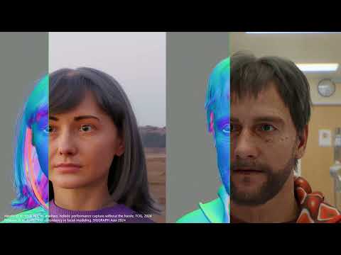
Our human-centric dense prediction model delivers high-quality, detailed (depth) results while achieving remarkable efficiency, running orders of magnitude faster than competing methods, with inference speeds as low as 21 milliseconds per frame (the large multi-task model on an NVIDIA A100). It reliably captures a wide range of human characteristics under diverse lighting conditions, preserving fine-grained details such as hair strands and subtle facial features. This demonstrates the model’s robustness and accuracy in complex, real-world scenarios.
The state of the art in human-centric computer vision achieves high accuracy and robustness across a diverse range of tasks. The most effective models in this domain have billions of parameters, thus requiring extremely large datasets, expensive training regimes, and compute-intensive inference. In this paper, we demonstrate that it is possible to train models on much smaller but high-fidelity synthetic datasets, with no loss in accuracy and higher efficiency. Using synthetic training data provides us with excellent levels of detail and perfect labels, while providing strong guarantees for data provenance, usage rights, and user consent. Procedural data synthesis also provides us with explicit control on data diversity, that we can use to address unfairness in the models we train. Extensive quantitative assessment on real input images demonstrates accuracy of our models on three dense prediction tasks: depth estimation, surface normal estimation, and soft foreground segmentation. Our models require only a fraction of the cost of training and inference when compared with foundational models of similar accuracy.
QuickTime (.mov) files are fundamentally time-based, not frame-based, and so don’t have a built-in, uniform “first frame/last frame” field you can set as numeric frame IDs. Instead, tools like Shotgun Create rely on the timecode track and the movie’s duration to infer frame numbers. If you want Shotgun to pick up a non-default frame range (e.g. start at 1001, end at 1064), you must bake in an SMPTE timecode that corresponds to your desired start frame, and ensure the movie’s duration matches your clip length.
How Shotgun Reads Frame Ranges
Default start frame is 1. If no timecode metadata is present, Shotgun assumes the movie begins at frame 1.
Timecode ⇒ frame number. Shotgun Create “honors the timecodes of media sources,” mapping the embedded TC to frame IDs. For example, a 24 fps QuickTime tagged with a start timecode of 00:00:41:17 will be interpreted as beginning on frame 1001 (1001 ÷ 24 fps ≈ 41.71 s).
Embedding a Start Timecode
QuickTime uses a tmcd (timecode) track. You can bake in an SMPTE track via FFmpeg’s -timecode flag or via Compressor/encoder settings:
Compute your start TC.
Desired start frame = 1001
Frame 1001 at 24 fps ⇒ 1001 ÷ 24 ≈ 41.708 s ⇒ TC 00:00:41:17
Aider enables developers to interactively generate, modify, and test code by leveraging both cloud-hosted and local LLMs directly from the terminal or within an IDE. Key capabilities include comprehensive codebase mapping, support for over 100 programming languages, automated git commit messages, voice-to-code interactions, and built-in linting and testing workflows. Installation is straightforward via pip or uv, and while the tool itself has no licensing cost, actual usage costs stem from the underlying LLM APIs, which are billed separately by providers like OpenAI or Anthropic.
Key Features
Cloud & Local LLM Support Connect to most major LLM providers out of the box, or run models locally for privacy and cost control aider.chat.
Codebase Mapping Automatically indexes all project files so that even large repositories can be edited contextually aider.chat.
100+ Language Support Works with Python, JavaScript, Rust, Ruby, Go, C++, PHP, HTML, CSS, and dozens more aider.chat.
Git Integration Generates sensible commit messages and automates diffs/undo operations through familiar git tooling aider.chat.
Voice-to-Code Speak commands to Aider to request features, tests, or fixes without typing aider.chat.
Images & Web Pages Attach screenshots, diagrams, or documentation URLs to provide visual context for edits aider.chat.
Linting & Testing Runs lint and test suites automatically after each change, and can fix issues it detects
Sourcetree and GitHub Desktop are both free, GUI-based Git clients aimed at simplifying version control for developers. While they share the same core purpose—making Git more accessible—they differ in features, UI design, integration options, and target audiences.
An exposure stop is a unit measurement of Exposure as such it provides a universal linear scale to measure the increase and decrease in light, exposed to the image sensor, due to changes in shutter speed, iso and f-stop.
+-1 stop is a doubling or halving of the amount of light let in when taking a photo
1 EV (exposure value) is just another way to say one stop of exposure change.
Same applies to shutter speed, iso and aperture.
Doubling or halving your shutter speed produces an increase or decrease of 1 stop of exposure.
Doubling or halving your iso speed produces an increase or decrease of 1 stop of exposure.
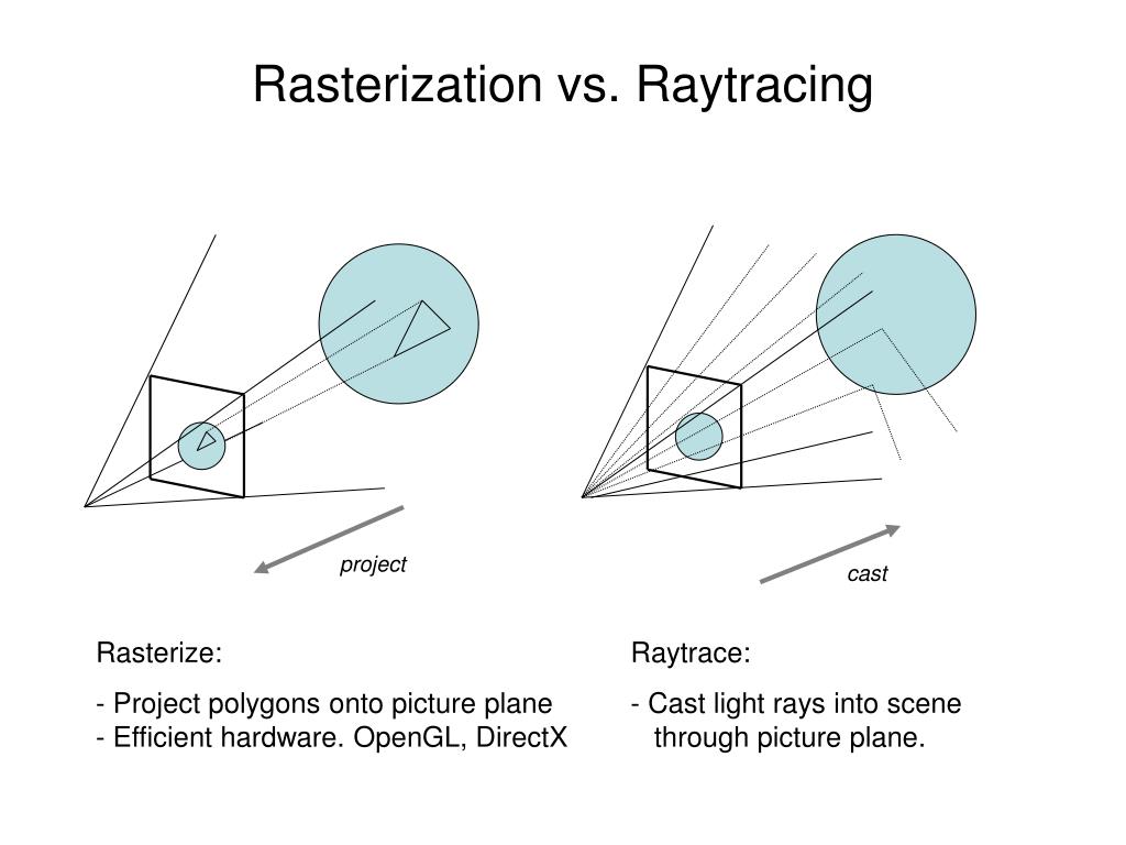
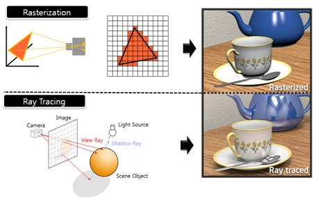
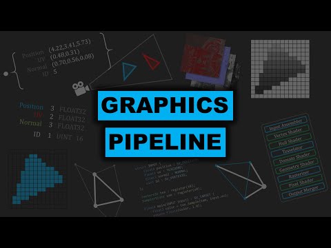
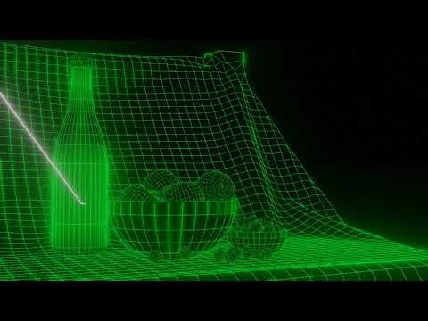
RASTERIZATION Rasterisation (or rasterization) is the task of taking the information described in a vector graphics format OR the vertices of triangles making 3D shapes and converting them into a raster image (a series of pixels, dots or lines, which, when displayed together, create the image which was represented via shapes), or in other words “rasterizing” vectors or 3D models onto a 2D plane for display on a computer screen.
For each triangle of a 3D shape, you project the corners of the triangle on the virtual screen with some math (projective geometry). Then you have the position of the 3 corners of the triangle on the pixel screen. Those 3 points have texture coordinates, so you know where in the texture are the 3 corners. The cost is proportional to the number of triangles, and is only a little bit affected by the screen resolution.
In computer graphics, a raster graphics orbitmap image is a dot matrix data structure that represents a generally rectangular grid of pixels (points of color), viewable via a monitor, paper, or other display medium.
With rasterization, objects on the screen are created from a mesh of virtual triangles, or polygons, that create 3D models of objects. A lot of information is associated with each vertex, including its position in space, as well as information about color, texture and its “normal,” which is used to determine the way the surface of an object is facing.
Computers then convert the triangles of the 3D models into pixels, or dots, on a 2D screen. Each pixel can be assigned an initial color value from the data stored in the triangle vertices.
Further pixel processing or “shading,” including changing pixel color based on how lights in the scene hit the pixel, and applying one or more textures to the pixel, combine to generate the final color applied to a pixel.
The main advantage of rasterization is its speed. However, rasterization is simply the process of computing the mapping from scene geometry to pixels and does not prescribe a particular way to compute the color of those pixels. So it cannot take shading, especially the physical light, into account and it cannot promise to get a photorealistic output. That’s a big limitation of rasterization.
There are also multiple problems:
If you have two triangles one is behind the other, you will draw twice all the pixels. you only keep the pixel from the triangle that is closer to you (Z-buffer), but you still do the work twice.
The borders of your triangles are jagged as it is hard to know if a pixel is in the triangle or out. You can do some smoothing on those, that is anti-aliasing.
You have to handle every triangles (including the ones behind you) and then see that they do not touch the screen at all. (we have techniques to mitigate this where we only look at triangles that are in the field of view)
Transparency is hard to handle (you can’t just do an average of the color of overlapping transparent triangles, you have to do it in the right order)
RAY CASTING It is almost the exact reverse of rasterization: you start from the virtual screen instead of the vector or 3D shapes, and you project a ray, starting from each pixel of the screen, until it intersect with a triangle.
The cost is directly correlated to the number of pixels in the screen and you need a really cheap way of finding the first triangle that intersect a ray. In the end, it is more expensive than rasterization but it will, by design, ignore the triangles that are out of the field of view.
You can use it to continue after the first triangle it hit, to take a little bit of the color of the next one, etc… This is useful to handle the border of the triangle cleanly (less jagged) and to handle transparency correctly.
RAYTRACING
Same idea as ray casting except once you hit a triangle you reflect on it and go into a different direction. The number of reflection you allow is the “depth” of your ray tracing. The color of the pixel can be calculated, based off the light source and all the polygons it had to reflect off of to get to that screen pixel.
The easiest way to think of ray tracing is to look around you, right now. The objects you’re seeing are illuminated by beams of light. Now turn that around and follow the path of those beams backwards from your eye to the objects that light interacts with. That’s ray tracing.
Ray tracing is eye-oriented process that needs walking through each pixel looking for what object should be shown there, which is also can be described as a technique that follows a beam of light (in pixels) from a set point and simulates how it reacts when it encounters objects.
Compared with rasterization, ray tracing is hard to be implemented in real time, since even one ray can be traced and processed without much trouble, but after one ray bounces off an object, it can turn into 10 rays, and those 10 can turn into 100, 1000…The increase is exponential, and the the calculation for all these rays will be time consuming.
Historically, computer hardware hasn’t been fast enough to use these techniques in real time, such as in video games. Moviemakers can take as long as they like to render a single frame, so they do it offline in render farms. Video games have only a fraction of a second. As a result, most real-time graphics rely on the another technique called rasterization.
PATH TRACING Path tracing can be used to solve more complex lighting situations. Path tracing is a type of ray tracing. When using path tracing for rendering, the rays only produce a single ray per bounce. The rays do not follow a defined line per bounce(to a light, for example), but rather shoot off in a random direction. The path tracing algorithm then takes a random sampling of all of the rays to create the final image. This results in sampling a variety of different types of lighting.
When a ray hits a surface it doesn’t trace a path to every light source, instead it bounces the ray off the surface and keeps bouncing it until it hits a light source or exhausts some bounce limit. It then calculates the amount of light transferred all the way to the pixel, including any color information gathered from surfaces along the way. It then averages out the values calculated from all the paths that were traced into the scene to get the final pixel color value.
It requires a ton of computing power and if you don’t send out enough rays per pixel or don’t trace the paths far enough into the scene then you end up with a very spotty image as many pixels fail to find any light sources from their rays. So when you increase the the samples per pixel, you can see the image quality becomes better and better.
Ray tracing tends to be more efficient than path tracing. Basically, the render time of a ray tracer depends on the number of polygons in the scene. The more polygons you have, the longer it will take. Meanwhile, the rendering time of a path tracer can be indifferent to the number of polygons, but it is related to light situation: If you add a light, transparency, translucence, or other shader effects, the path tracer will slow down considerably.
Spectral sensitivity of eye is influenced by light intensity. And the light intensity determines the level of activity of cones cell and rod cell. This is the main characteristic of human vision. Sensitivity to individual colors, in other words, wavelengths of the light spectrum, is explained by the RGB (red-green-blue) theory. This theory assumed that there are three kinds of cones. It’s selectively sensitive to red (700-630 nm), green (560-500 nm), and blue (490-450 nm) light. And their mutual interaction allow to perceive all colors of the spectrum.
The Manuka rendering architecture has been designed in the spirit of the classic reyes rendering architecture. In its core, reyes is based on stochastic rasterisation of micropolygons, facilitating depth of field, motion blur, high geometric complexity,and programmable shading.
This is commonly achieved with Monte Carlo path tracing, using a paradigm often called shade-on-hit, in which the renderer alternates tracing rays with running shaders on the various ray hits. The shaders take the role of generating the inputs of the local material structure which is then used bypath sampling logic to evaluate contributions and to inform what further rays to cast through the scene.
Over the years, however, the expectations have risen substantially when it comes to image quality. Computing pictures which are indistinguishable from real footage requires accurate simulation of light transport, which is most often performed using some variant of Monte Carlo path tracing. Unfortunately this paradigm requires random memory accesses to the whole scene and does not lend itself well to a rasterisation approach at all.
Manuka is both a uni-directional and bidirectional path tracer and encompasses multiple importance sampling (MIS). Interestingly, and importantly for production character skin work, it is the first major production renderer to incorporate spectral MIS in the form of a new ‘Hero Spectral Sampling’ technique, which was recently published at Eurographics Symposium on Rendering 2014.
Manuka propose a shade-before-hit paradigm in-stead and minimise I/O strain (and some memory costs) on the system, leveraging locality of reference by running pattern generation shaders before we execute light transport simulation by path sampling, “compressing” any bvh structure as needed, and as such also limiting duplication of source data.
The difference with reyes is that instead of baking colors into the geometry like in Reyes, manuka bakes surface closures. This means that light transport is still calculated with path tracing, but all texture lookups etc. are done up-front and baked into the geometry.
The main drawback with this method is that geometry has to be tessellated to its highest, stable topology before shading can be evaluated properly. As such, the high cost to first pixel. Even a basic 4 vertices square becomes a much more complex model with this approach.
Manuka use the RenderMan Shading Language (rsl) for programmable shading [Pixar Animation Studios 2015], but we do not invoke rsl shaders when intersecting a ray with a surface (often called shade-on-hit). Instead, we pre-tessellate and pre-shade all the input geometry in the front end of the renderer.
This way, we can efficiently order shading computations to sup-port near-optimal texture locality, vectorisation, and parallelism. This system avoids repeated evaluation of shaders at the same surface point, and presents a minimal amount of memory to be accessed during light transport time. An added benefit is that the acceleration structure for ray tracing (abounding volume hierarchy, bvh) is built once on the final tessellated geometry, which allows us to ray trace more efficiently than multi-level bvhs and avoids costly caching of on-demand tessellated micropolygons and the associated scheduling issues.
For the shading reasons above, in terms of AOVs, the studio approach is to succeed at combining complex shading with ray paths in the render rather than pass a multi-pass render to compositing.
For the Spectral Rendering component. The light transport stage is fully spectral, using a continuously sampled wavelength which is traced with each path and used to apply the spectral camera sensitivity of the sensor. This allows for faithfully support any degree of observer metamerism as the camera footage they are intended to match as well as complex materials which require wavelength dependent phenomena such as diffraction, dispersion, interference, iridescence, or chromatic extinction and Rayleigh scattering in participating media.
As opposed to the original reyes paper, we use bilinear interpolation of these bsdf inputs later when evaluating bsdfs per pathv ertex during light transport4. This improves temporal stability of geometry which moves very slowly with respect to the pixel raster
In terms of the pipeline, everything rendered at Weta was already completely interwoven with their deep data pipeline. Manuka very much was written with deep data in mind. Here, Manuka not so much extends the deep capabilities, rather it fully matches the already extremely complex and powerful setup Weta Digital already enjoy with RenderMan. For example, an ape in a scene can be selected, its ID is available and a NUKE artist can then paint in 3D say a hand and part of the way up the neutral posed ape.
We called our system Manuka, as a respectful nod to reyes: we had heard a story froma former ILM employee about how reyes got its name from how fond the early Pixar people were of their lunches at Point Reyes, and decided to name our system after our surrounding natural environment, too. Manuka is a kind of tea tree very common in New Zealand which has very many very small leaves, in analogy to micropolygons ina tree structure for ray tracing. It also happens to be the case that Weta Digital’s main site is on Manuka Street.


