


COMPOSITION
DESIGN


COLOR
-
GretagMacbeth Color Checker Numeric Values and Middle Gray
Read more: GretagMacbeth Color Checker Numeric Values and Middle GrayThe human eye perceives half scene brightness not as the linear 50% of the present energy (linear nature values) but as 18% of the overall brightness. We are biased to perceive more information in the dark and contrast areas. A Macbeth chart helps with calibrating back into a photographic capture into this “human perspective” of the world.
https://en.wikipedia.org/wiki/Middle_gray
In photography, painting, and other visual arts, middle gray or middle grey is a tone that is perceptually about halfway between black and white on a lightness scale in photography and printing, it is typically defined as 18% reflectance in visible light

Light meters, cameras, and pictures are often calibrated using an 18% gray card[4][5][6] or a color reference card such as a ColorChecker. On the assumption that 18% is similar to the average reflectance of a scene, a grey card can be used to estimate the required exposure of the film.
https://en.wikipedia.org/wiki/ColorChecker
(more…) -
PBR Color Reference List for Materials – by Grzegorz Baran
Read more: PBR Color Reference List for Materials – by Grzegorz Baran
“The list should be helpful for every material artist who work on PBR materials as it contains over 200 color values measured with PCE-RGB2 1002 Color Spectrometer device and presented in linear and sRGB (2.2) gamma space.
All color values, HUE and Saturation in this list come from measurements taken with PCE-RGB2 1002 Color Spectrometer device and are presented in linear and sRGB (2.2) gamma space (more info at the end of this video) I calculated Relative Luminance and Luminance values based on captured color using my own equation which takes color based luminance perception into consideration. Bare in mind that there is no ‘one’ color per substance as nothing in nature is even 100% uniform and any value in +/-10% range from these should be considered as correct one. Therefore this list should be always considered as a color reference for material’s albedos, not ulitimate and absolute truth.“
-
About color: What is a LUT
Read more: About color: What is a LUThttp://www.lightillusion.com/luts.html
https://www.shutterstock.com/blog/how-use-luts-color-grading
A LUT (Lookup Table) is essentially the modifier between two images, the original image and the displayed image, based on a mathematical formula. Basically conversion matrices of different complexities. There are different types of LUTS – viewing, transform, calibration, 1D and 3D.


-
Tobia Montanari – Memory Colors: an essential tool for Colorists
Read more: Tobia Montanari – Memory Colors: an essential tool for Coloristshttps://www.tobiamontanari.com/memory-colors-an-essential-tool-for-colorists/
“Memory colors are colors that are universally associated with specific objects, elements or scenes in our environment. They are the colors that we expect to see in specific situations: these colors are based on our expectation of how certain objects should look based on our past experiences and memories.
For instance, we associate specific hues, saturation and brightness values with human skintones and a slight variation can significantly affect the way we perceive a scene.
Similarly, we expect blue skies to have a particular hue, green trees to be a specific shade and so on.
Memory colors live inside of our brains and we often impose them onto what we see. By considering them during the grading process, the resulting image will be more visually appealing and won’t distract the viewer from the intended message of the story. Even a slight deviation from memory colors in a movie can create a sense of discordance, ultimately detracting from the viewer’s experience.”


LIGHTING
-
Photography basics: Solid Angle measures
Read more: Photography basics: Solid Angle measureshttp://www.calculator.org/property.aspx?name=solid+angle

A measure of how large the object appears to an observer looking from that point. Thus. A measure for objects in the sky. Useful to retuen the size of the sun and moon… and in perspective, how much of their contribution to lighting. Solid angle can be represented in ‘angular diameter’ as well.
http://en.wikipedia.org/wiki/Solid_angle
http://www.mathsisfun.com/geometry/steradian.html
A solid angle is expressed in a dimensionless unit called a steradian (symbol: sr). By default in terms of the total celestial sphere and before atmospheric’s scattering, the Sun and the Moon subtend fractional areas of 0.000546% (Sun) and 0.000531% (Moon).
http://en.wikipedia.org/wiki/Solid_angle#Sun_and_Moon
On earth the sun is likely closer to 0.00011 solid angle after athmospheric scattering. The sun as perceived from earth has a diameter of 0.53 degrees. This is about 0.000064 solid angle.
http://www.numericana.com/answer/angles.htm
The mean angular diameter of the full moon is 2q = 0.52° (it varies with time around that average, by about 0.009°). This translates into a solid angle of 0.0000647 sr, which means that the whole night sky covers a solid angle roughly one hundred thousand times greater than the full moon.
More info
http://lcogt.net/spacebook/using-angles-describe-positions-and-apparent-sizes-objects
http://amazing-space.stsci.edu/glossary/def.php.s=topic_astronomy
Angular Size
The apparent size of an object as seen by an observer; expressed in units of degrees (of arc), arc minutes, or arc seconds. The moon, as viewed from the Earth, has an angular diameter of one-half a degree.
The angle covered by the diameter of the full moon is about 31 arcmin or 1/2°, so astronomers would say the Moon’s angular diameter is 31 arcmin, or the Moon subtends an angle of 31 arcmin.

-
How to Direct and Edit a Fight Scene for Rhythm and Pacing
Read more: How to Direct and Edit a Fight Scene for Rhythm and Pacingwww.premiumbeat.com/blog/directing-fight-scene-cinematography/

1- Frame the action
2- Stage the action
3- Use camera movements
4- Set a rhythm
5- Control the speed of the action
-
Is a MacBeth Colour Rendition Chart the Safest Way to Calibrate a Camera?
Read more: Is a MacBeth Colour Rendition Chart the Safest Way to Calibrate a Camera?www.colour-science.org/posts/the-colorchecker-considered-mostly-harmless/
“Unless you have all the relevant spectral measurements, a colour rendition chart should not be used to perform colour-correction of camera imagery but only for white balancing and relative exposure adjustments.”
“Using a colour rendition chart for colour-correction might dramatically increase error if the scene light source spectrum is different from the illuminant used to compute the colour rendition chart’s reference values.”
“other factors make using a colour rendition chart unsuitable for camera calibration:
– Uncontrolled geometry of the colour rendition chart with the incident illumination and the camera.
– Unknown sample reflectances and ageing as the colour of the samples vary with time.
– Low samples count.
– Camera noise and flare.
– Etc…“Those issues are well understood in the VFX industry, and when receiving plates, we almost exclusively use colour rendition charts to white balance and perform relative exposure adjustments, i.e. plate neutralisation.”
-
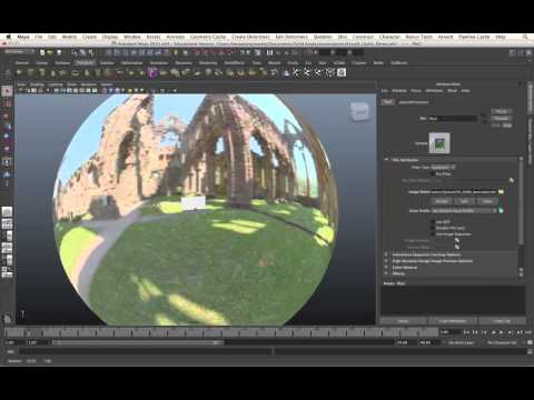
RawTherapee – a free, open source, cross-platform raw image and HDRi processing program
Read more: RawTherapee – a free, open source, cross-platform raw image and HDRi processing program5.10 of this tool includes excellent tools to clean up cr2 and cr3 used on set to support HDRI processing.
Converting raw to AcesCG 32 bit tiffs with metadata.


COLLECTIONS
| Featured AI
| Design And Composition
| Explore posts
POPULAR SEARCHES
unreal | pipeline | virtual production | free | learn | photoshop | 360 | macro | google | nvidia | resolution | open source | hdri | real-time | photography basics | nuke
FEATURED POSTS
Social Links
DISCLAIMER – Links and images on this website may be protected by the respective owners’ copyright. All data submitted by users through this site shall be treated as freely available to share.
