The intricate relationship between the eyes and the brain, often termed the eye-mind connection, reveals that vision is predominantly a cognitive process. This understanding has profound implications for fields such as design, where capturing and maintaining attention is paramount. This essay delves into the nuances of visual perception, the brain’s role in interpreting visual data, and how this knowledge can be applied to effective design strategies.
This cognitive aspect of vision is evident in phenomena such as optical illusions, where the brain interprets visual information in a way that contradicts physical reality. These illusions underscore that what we “see” is not merely a direct recording of the external world but a constructed experience shaped by cognitive processes.
Understanding the cognitive nature of vision is crucial for effective design. Designers must consider how the brain processes visual information to create compelling and engaging visuals. This involves several key principles:
Note: In Foundry’s Nuke, the software will map 18% gray to whatever your center f/stop is set to in the viewer settings (f/8 by default… change that to EV by following the instructions below).
You can experiment with this by attaching an Exposure node to a Constant set to 0.18, setting your viewer read-out to Spotmeter, and adjusting the stops in the node up and down. You will see that a full stop up or down will give you the respective next value on the aperture scale (f8, f11, f16 etc.).
One stop doubles or halves the amount or light that hits the filmback/ccd, so everything works in powers of 2.
So starting with 0.18 in your constant, you will see that raising it by a stop will give you .36 as a floating point number (in linear space), while your f/stop will be f/11 and so on.
If you set your center stop to 0 (see below) you will get a relative readout in EVs, where EV 0 again equals 18% constant gray.
In other words. Setting the center f-stop to 0 means that in a neutral plate, the middle gray in the macbeth chart will equal to exposure value 0. EV 0 corresponds to an exposure time of 1 sec and an aperture of f/1.0.
This will set the sun usually around EV12-17 and the sky EV1-4 , depending on cloud coverage.
To switch Foundry’s Nuke’s SpotMeter to return the EV of an image, click on the main viewport, and then press s, this opens the viewer’s properties. Now set the center f-stop to 0 in there. And the SpotMeter in the viewport will change from aperture and fstops to EV.
Spectral sensitivity of eye is influenced by light intensity. And the light intensity determines the level of activity of cones cell and rod cell. This is the main characteristic of human vision. Sensitivity to individual colors, in other words, wavelengths of the light spectrum, is explained by the RGB (red-green-blue) theory. This theory assumed that there are three kinds of cones. It’s selectively sensitive to red (700-630 nm), green (560-500 nm), and blue (490-450 nm) light. And their mutual interaction allow to perceive all colors of the spectrum.
While the human eye has red, green, and blue-sensing cones, those cones are cross-wired in the retina to produce a luminance channel plus a red-green and a blue-yellow channel, and it’s data in that color space (known technically as “LAB”) that goes to the brain. That’s why we can’t perceive a reddish-green or a yellowish-blue, whereas such colors can be represented in the RGB color space used by digital cameras.
The back of the retina is covered in light-sensitive neurons known as cone cells and rod cells. There are three types of cone cells, each sensitive to different ranges of light. These ranges overlap, but for convenience the cones are referred to as blue (short-wavelength), green (medium-wavelength), and red (long-wavelength). The rod cells are primarily used in low-light situations, so we’ll ignore those for now.
When light enters the eye and hits the cone cells, the cones get excited and send signals to the brain through the visual cortex. Different wavelengths of light excite different combinations of cones to varying levels, which generates our perception of color. You can see that the red cones are most sensitive to light, and the blue cones are least sensitive. The sensitivity of green and red cones overlaps for most of the visible spectrum.
Here’s how your brain takes the signals of light intensity from the cones and turns it into color information. To see red or green, your brain finds the difference between the levels of excitement in your red and green cones. This is the red-green channel.
To get “brightness,” your brain combines the excitement of your red and green cones. This creates the luminance, or black-white, channel. To see yellow or blue, your brain then finds the difference between this luminance signal and the excitement of your blue cones. This is the yellow-blue channel.
From the calculations made in the brain along those three channels, we get four basic colors: blue, green, yellow, and red. Seeing blue is what you experience when low-wavelength light excites the blue cones more than the green and red.
Seeing green happens when light excites the green cones more than the red cones. Seeing red happens when only the red cones are excited by high-wavelength light.
Here’s where it gets interesting. Seeing yellow is what happens when BOTH the green AND red cones are highly excited near their peak sensitivity. This is the biggest collective excitement that your cones ever have, aside from seeing pure white.
Notice that yellow occurs at peak intensity in the graph to the right. Further, the lens and cornea of the eye happen to block shorter wavelengths, reducing sensitivity to blue and violet light.
In HD we often refer to the range of available colors as a color gamut. Such a color gamut is typically plotted on a two-dimensional diagram, called a CIE chart, as shown in at the top of this blog. Each color is characterized by its x/y coordinates.
Good enough for government work, perhaps. But for HDR, with its higher luminance levels and wider color, the gamut becomes three-dimensional.
For HDR the color gamut therefore becomes a characteristic we now call the color volume. It isn’t easy to show color volume on a two-dimensional medium like the printed page or a computer screen, but one method is shown below. As the luminance becomes higher, the picture eventually turns to white. As it becomes darker, it fades to black. The traditional color gamut shown on the CIE chart is simply a slice through this color volume at a selected luminance level, such as 50%.
Three different color volumes—we still refer to them as color gamuts though their third dimension is important—are currently the most significant. The first is BT.709 (sometimes referred to as Rec.709), the color gamut used for pre-UHD/HDR formats, including standard HD.
The largest is known as BT.2020; it encompasses (roughly) the range of colors visible to the human eye (though ET might find it insufficient!).
Between these two is the color gamut used in digital cinema, known as DCI-P3.
“Memory colors are colors that are universally associated with specific objects, elements or scenes in our environment. They are the colors that we expect to see in specific situations: these colors are based on our expectation of how certain objects should look based on our past experiences and memories.
For instance, we associate specific hues, saturation and brightness values with human skintones and a slight variation can significantly affect the way we perceive a scene.
Similarly, we expect blue skies to have a particular hue, green trees to be a specific shade and so on.
Memory colors live inside of our brains and we often impose them onto what we see. By considering them during the grading process, the resulting image will be more visually appealing and won’t distract the viewer from the intended message of the story. Even a slight deviation from memory colors in a movie can create a sense of discordance, ultimately detracting from the viewer’s experience.”
This 2025 I decided to start learning how to code, so I installed Visual Studio and I started looking into C++. After days of watching tutorials and guides about the basics of C++ and programming, I decided to make something physics-related. I started with a dot that fell to the ground and then I wanted to simulate gravitational attraction, so I made 2 circles attracting each other. I thought it was really cool to see something I made with code actually work, so I kept building on top of that small, basic program. And here we are after roughly 8 months of learning programming. This is Galaxy Engine, and it is a simulation software I have been making ever since I started my learning journey. It currently can simulate gravity, dark matter, galaxies, the Big Bang, temperature, fluid dynamics, breakable solids, planetary interactions, etc. The program can run many tens of thousands of particles in real time on the CPU thanks to the Barnes-Hut algorithm, mixed with Morton curves. It also includes its own PBR 2D path tracer with BVH optimizations. The path tracer can simulate a bunch of stuff like diffuse lighting, specular reflections, refraction, internal reflection, fresnel, emission, dispersion, roughness, IOR, nested IOR and more! I tried to make the path tracer closer to traditional 3D render engines like V-Ray. I honestly never imagined I would go this far with programming, and it has been an amazing learning experience so far. I think that mixing this knowledge with my 3D knowledge can unlock countless new possibilities. In case you are curious about Galaxy Engine, I made it completely free and Open-Source so that anyone can build and compile it locally! You can find the source code inGitHub
import math,sys

def Exposure2Intensity(exposure):
    exp = float(exposure)
    result = math.pow(2,exp)
    print(result)

Exposure2Intensity(0)

def Intensity2Exposure(intensity):
    inarg = float(intensity)

    if inarg == 0:
        print("Exposure of zero intensity is undefined.")
        return

    if inarg < 1e-323:
        inarg = max(inarg, 1e-323)
        print("Exposure of negative intensities is undefined. Clamping to a very small value instead (1e-323)")

    result = math.log(inarg, 2)
    print(result)

Intensity2Exposure(0.1)
Why Exposure?
Exposure is a stop value that multiplies the intensity by 2 to the power of the stop. Increasing exposure by 1 results in double the amount of light.
Artists think in “stops.” Doubling or halving brightness is easy math and common in grading and look-dev. Exposure counts doublings in whole stops:
+1 stop = ×2 brightness
−1 stop = ×0.5 brightness
This gives perceptually even controls across both bright and dark values.
Why Intensity?
Intensity is linear. It’s what render engines and compositors expect when:
Summing values
Averaging pixels
Multiplying or filtering pixel data
Use intensity when you need the actual math on pixel/light data.
Formulas (from your Python)
Intensity from exposure: intensity = 2**exposure
Exposure from intensity: exposure = log₂(intensity)
Guardrails:
Intensity must be > 0 to compute exposure.
If intensity = 0 → exposure is undefined.
Clamp tiny values (e.g. 1e−323) before using log₂.
Use Exposure (stops) when…
You want artist-friendly sliders (−5…+5 stops)
Adjusting look-dev or grading in even stops
Matching plates with quick ±1 stop tweaks
Tweening brightness changes smoothly across ranges
Use Intensity (linear) when…
Storing raw pixel/light values
Multiplying textures or lights by a gain
Performing sums, averages, and filters
Feeding values to render engines expecting linear data
Examples
+2 stops → 2**2 = 4.0 (×4)
+1 stop → 2**1 = 2.0 (×2)
0 stop → 2**0 = 1.0 (×1)
−1 stop → 2**(−1) = 0.5 (×0.5)
−2 stops → 2**(−2) = 0.25 (×0.25)
Intensity 0.1 → exposure = log₂(0.1) ≈ −3.32
Rule of thumb
Think in stops (exposure) for controls and matching. Compute in linear (intensity) for rendering and math.
An open, Interactive 3D Design Collaboration Platform for Multi-Tool Workflows to simplify studio workflows for real-time graphics.
It supports Pixar’s Universal Scene Description technology for exchanging information about modeling, shading, animation, lighting, visual effects and rendering across multiple applications.
It also supports NVIDIA’s Material Definition Language, which allows artists to exchange information about surface materials across multiple tools.
With Omniverse, artists can see live updates made by other artists working in different applications. They can also see changes reflected in multiple tools at the same time.
For example an artist using Maya with a portal to Omniverse can collaborate with another artist using UE4 and both will see live updates of each others’ changes in their application.
DISCLAIMER – Links and images on this website may be protected by the respective owners’ copyright. All data submitted by users through this site shall be treated as freely available to share.


