


COMPOSITION
-
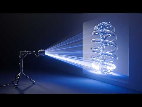
Composition – 5 tips for creating perfect cinematic lighting and making your work look stunning
Read more: Composition – 5 tips for creating perfect cinematic lighting and making your work look stunning
http://www.diyphotography.net/5-tips-creating-perfect-cinematic-lighting-making-work-look-stunning/
1. Learn the rules of lighting
2. Learn when to break the rules
3. Make your key light larger
4. Reverse keying
5. Always be backlighting
-
7 Commandments of Film Editing and composition
Read more: 7 Commandments of Film Editing and composition
1. Watch every frame of raw footage twice. On the second time, take notes. If you don’t do this and try to start developing a scene premature, then it’s a big disservice to yourself and to the director, actors and production crew.
2. Nurture the relationships with the director. You are the secondary person in the relationship. Be calm and continually offer solutions. Get the main intention of the film as soon as possible from the director.
3. Organize your media so that you can find any shot instantly.
4. Factor in extra time for renders, exports, errors and crashes.
5. Attempt edits and ideas that shouldn’t work. It just might work. Until you do it and watch it, you won’t know. Don’t rule out ideas just because they don’t make sense in your mind.
6. Spend more time on your audio. It’s the glue of your edit. AUDIO SAVES EVERYTHING. Create fluid and seamless audio under your video.
7. Make cuts for the scene, but always in context for the whole film. Have a macro and a micro view at all times.


DESIGN
-
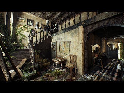
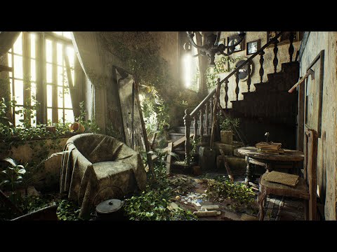
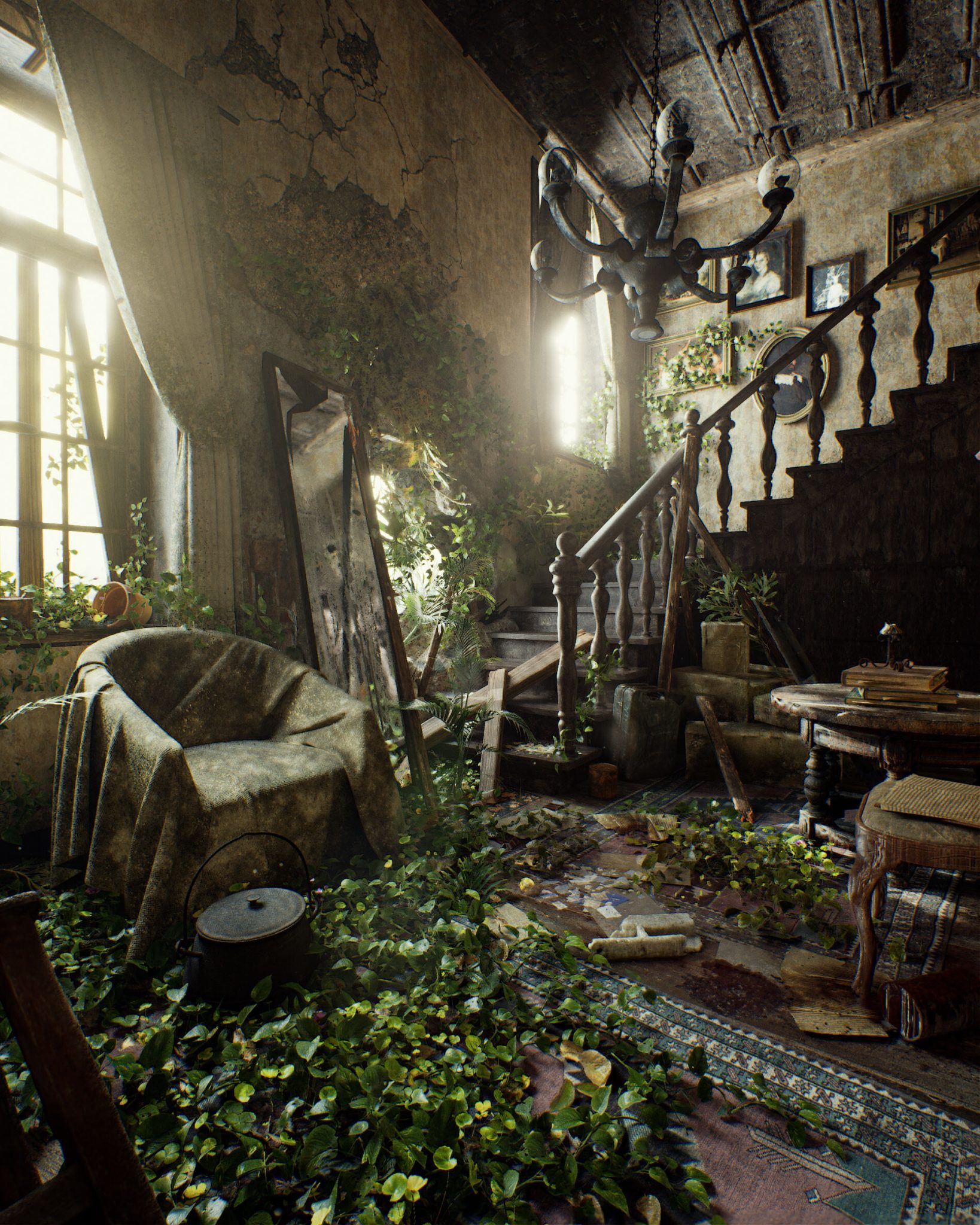
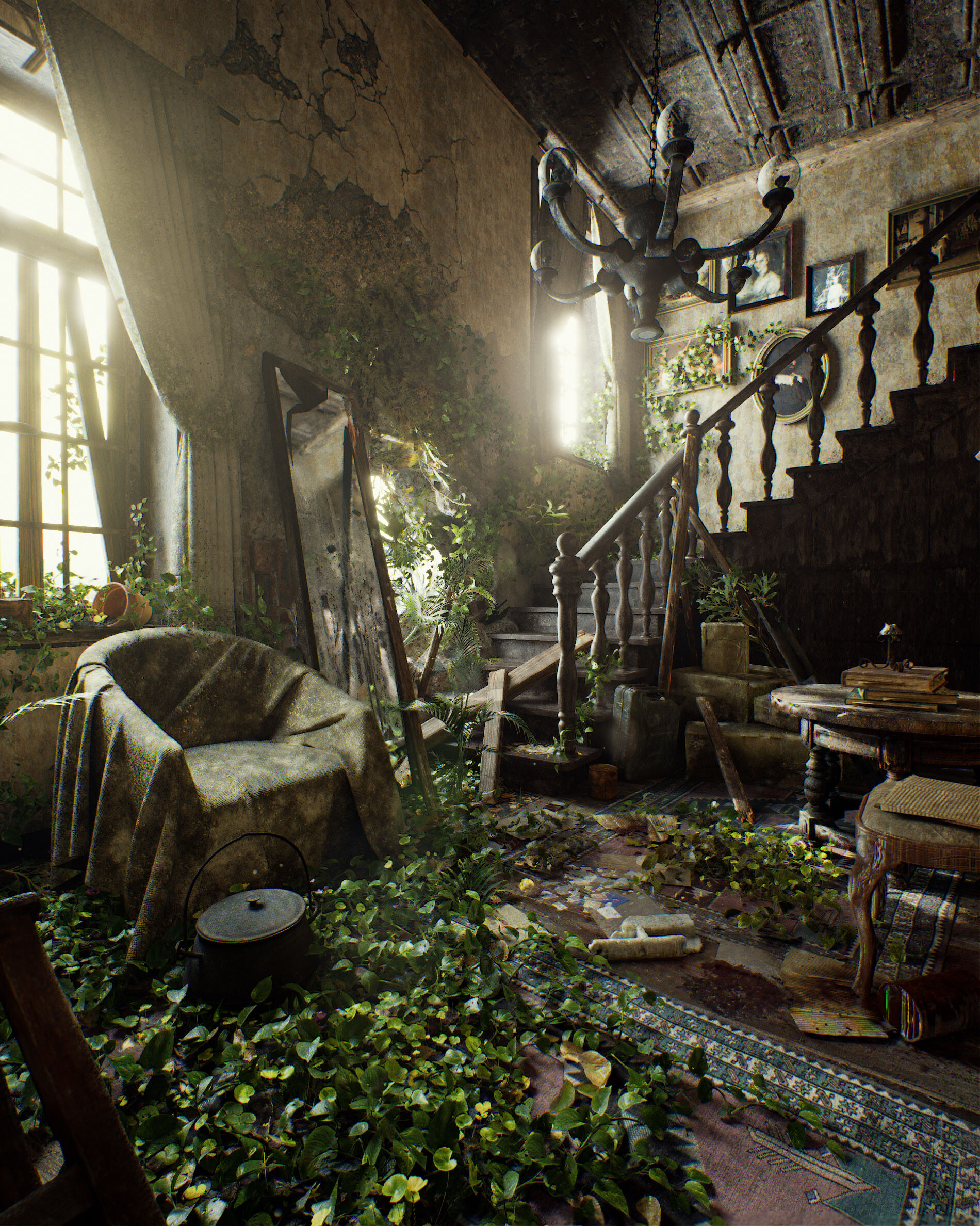
Pasquale Scionti – Production Walkthrough with Virtual Camera and iPad pro 11.5 on Unreal Engine 4.25
Read more: Pasquale Scionti – Production Walkthrough with Virtual Camera and iPad pro 11.5 on Unreal Engine 4.2580.lv/articles/creating-an-old-abandoned-mansion-with-quixel-tools/
www.artstation.com/artwork/Poexyo


COLOR
-
SecretWeapons MixBox – a practical library for paint-like digital color mixing
Read more: SecretWeapons MixBox – a practical library for paint-like digital color mixingInternally, Mixbox treats colors as real-life pigments using the Kubelka & Munk theory to predict realistic color behavior.
https://scrtwpns.com/mixbox/painter/
https://scrtwpns.com/mixbox.pdf
https://github.com/scrtwpns/mixbox
https://scrtwpns.com/mixbox/docs/

-
Photography Basics : Spectral Sensitivity Estimation Without a Camera
Read more: Photography Basics : Spectral Sensitivity Estimation Without a Camerahttps://color-lab-eilat.github.io/Spectral-sensitivity-estimation-web/
A number of problems in computer vision and related fields would be mitigated if camera spectral sensitivities were known. As consumer cameras are not designed for high-precision visual tasks, manufacturers do not disclose spectral sensitivities. Their estimation requires a costly optical setup, which triggered researchers to come up with numerous indirect methods that aim to lower cost and complexity by using color targets. However, the use of color targets gives rise to new complications that make the estimation more difficult, and consequently, there currently exists no simple, low-cost, robust go-to method for spectral sensitivity estimation that non-specialized research labs can adopt. Furthermore, even if not limited by hardware or cost, researchers frequently work with imagery from multiple cameras that they do not have in their possession.
To provide a practical solution to this problem, we propose a framework for spectral sensitivity estimation that not only does not require any hardware (including a color target), but also does not require physical access to the camera itself. Similar to other work, we formulate an optimization problem that minimizes a two-term objective function: a camera-specific term from a system of equations, and a universal term that bounds the solution space.
Different than other work, we utilize publicly available high-quality calibration data to construct both terms. We use the colorimetric mapping matrices provided by the Adobe DNG Converter to formulate the camera-specific system of equations, and constrain the solutions using an autoencoder trained on a database of ground-truth curves. On average, we achieve reconstruction errors as low as those that can arise due to manufacturing imperfections between two copies of the same camera. We provide predicted sensitivities for more than 1,000 cameras that the Adobe DNG Converter currently supports, and discuss which tasks can become trivial when camera responses are available.


-
Victor Perez – The Color Management Handbook for Visual Effects Artists
Read more: Victor Perez – The Color Management Handbook for Visual Effects ArtistsDigital Color Principles, Color Management Fundamentals & ACES Workflows

-
Photography basics: Why Use a (MacBeth) Color Chart?
Read more: Photography basics: Why Use a (MacBeth) Color Chart?Start here: https://www.pixelsham.com/2013/05/09/gretagmacbeth-color-checker-numeric-values/
https://www.studiobinder.com/blog/what-is-a-color-checker-tool/


In LightRoom

in Final Cut

in Nuke
Note: In Foundry’s Nuke, the software will map 18% gray to whatever your center f/stop is set to in the viewer settings (f/8 by default… change that to EV by following the instructions below).
You can experiment with this by attaching an Exposure node to a Constant set to 0.18, setting your viewer read-out to Spotmeter, and adjusting the stops in the node up and down. You will see that a full stop up or down will give you the respective next value on the aperture scale (f8, f11, f16 etc.).One stop doubles or halves the amount or light that hits the filmback/ccd, so everything works in powers of 2.
So starting with 0.18 in your constant, you will see that raising it by a stop will give you .36 as a floating point number (in linear space), while your f/stop will be f/11 and so on.If you set your center stop to 0 (see below) you will get a relative readout in EVs, where EV 0 again equals 18% constant gray.

In other words. Setting the center f-stop to 0 means that in a neutral plate, the middle gray in the macbeth chart will equal to exposure value 0. EV 0 corresponds to an exposure time of 1 sec and an aperture of f/1.0.
This will set the sun usually around EV12-17 and the sky EV1-4 , depending on cloud coverage.
To switch Foundry’s Nuke’s SpotMeter to return the EV of an image, click on the main viewport, and then press s, this opens the viewer’s properties. Now set the center f-stop to 0 in there. And the SpotMeter in the viewport will change from aperture and fstops to EV.
-
OpenColorIO standard
Read more: OpenColorIO standardhttps://www.provideocoalition.com/color-management-part-11-introducing-opencolorio/
OpenColorIO (OCIO) is a new open source project from Sony Imageworks.
Based on development started in 2003, OCIO enables color transforms and image display to be handled in a consistent manner across multiple graphics applications. Unlike other color management solutions, OCIO is geared towards motion-picture post production, with an emphasis on visual effects and animation color pipelines.

-
Composition – cinematography Cheat Sheet
Read more: Composition – cinematography Cheat Sheet
Where is our eye attracted first? Why?
Size. Focus. Lighting. Color.
Size. Mr. White (Harvey Keitel) on the right.
Focus. He’s one of the two objects in focus.
Lighting. Mr. White is large and in focus and Mr. Pink (Steve Buscemi) is highlighted by
a shaft of light.
Color. Both are black and white but the read on Mr. White’s shirt now really stands out.
(more…)
What type of lighting?


LIGHTING
-
Fast, optimized ‘for’ pixel loops with OpenCV and Python to create tone mapped HDR images
Read more: Fast, optimized ‘for’ pixel loops with OpenCV and Python to create tone mapped HDR imageshttps://pyimagesearch.com/2017/08/28/fast-optimized-for-pixel-loops-with-opencv-and-python/
https://learnopencv.com/exposure-fusion-using-opencv-cpp-python/
Exposure Fusion is a method for combining images taken with different exposure settings into one image that looks like a tone mapped High Dynamic Range (HDR) image.

-
What’s the Difference Between Ray Casting, Ray Tracing, Path Tracing and Rasterization? Physical light tracing…
Read more: What’s the Difference Between Ray Casting, Ray Tracing, Path Tracing and Rasterization? Physical light tracing…RASTERIZATION
Rasterisation (or rasterization) is the task of taking the information described in a vector graphics format OR the vertices of triangles making 3D shapes and converting them into a raster image (a series of pixels, dots or lines, which, when displayed together, create the image which was represented via shapes), or in other words “rasterizing” vectors or 3D models onto a 2D plane for display on a computer screen.For each triangle of a 3D shape, you project the corners of the triangle on the virtual screen with some math (projective geometry). Then you have the position of the 3 corners of the triangle on the pixel screen. Those 3 points have texture coordinates, so you know where in the texture are the 3 corners. The cost is proportional to the number of triangles, and is only a little bit affected by the screen resolution.
In computer graphics, a raster graphics or bitmap image is a dot matrix data structure that represents a generally rectangular grid of pixels (points of color), viewable via a monitor, paper, or other display medium.
With rasterization, objects on the screen are created from a mesh of virtual triangles, or polygons, that create 3D models of objects. A lot of information is associated with each vertex, including its position in space, as well as information about color, texture and its “normal,” which is used to determine the way the surface of an object is facing.
Computers then convert the triangles of the 3D models into pixels, or dots, on a 2D screen. Each pixel can be assigned an initial color value from the data stored in the triangle vertices.
Further pixel processing or “shading,” including changing pixel color based on how lights in the scene hit the pixel, and applying one or more textures to the pixel, combine to generate the final color applied to a pixel.
The main advantage of rasterization is its speed. However, rasterization is simply the process of computing the mapping from scene geometry to pixels and does not prescribe a particular way to compute the color of those pixels. So it cannot take shading, especially the physical light, into account and it cannot promise to get a photorealistic output. That’s a big limitation of rasterization.
There are also multiple problems:
If you have two triangles one is behind the other, you will draw twice all the pixels. you only keep the pixel from the triangle that is closer to you (Z-buffer), but you still do the work twice.
The borders of your triangles are jagged as it is hard to know if a pixel is in the triangle or out. You can do some smoothing on those, that is anti-aliasing.
You have to handle every triangles (including the ones behind you) and then see that they do not touch the screen at all. (we have techniques to mitigate this where we only look at triangles that are in the field of view)
Transparency is hard to handle (you can’t just do an average of the color of overlapping transparent triangles, you have to do it in the right order)
-
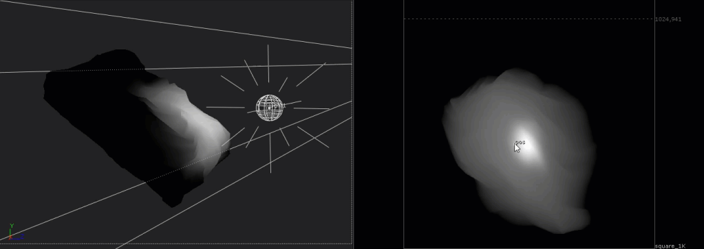
DiffusionLight: HDRI Light Probes for Free by Painting a Chrome Ball
Read more: DiffusionLight: HDRI Light Probes for Free by Painting a Chrome Ballhttps://diffusionlight.github.io/
https://github.com/DiffusionLight/DiffusionLight
https://github.com/DiffusionLight/DiffusionLight?tab=MIT-1-ov-file#readme
https://colab.research.google.com/drive/15pC4qb9mEtRYsW3utXkk-jnaeVxUy-0S
“a simple yet effective technique to estimate lighting in a single input image. Current techniques rely heavily on HDR panorama datasets to train neural networks to regress an input with limited field-of-view to a full environment map. However, these approaches often struggle with real-world, uncontrolled settings due to the limited diversity and size of their datasets. To address this problem, we leverage diffusion models trained on billions of standard images to render a chrome ball into the input image. Despite its simplicity, this task remains challenging: the diffusion models often insert incorrect or inconsistent objects and cannot readily generate images in HDR format. Our research uncovers a surprising relationship between the appearance of chrome balls and the initial diffusion noise map, which we utilize to consistently generate high-quality chrome balls. We further fine-tune an LDR difusion model (Stable Diffusion XL) with LoRA, enabling it to perform exposure bracketing for HDR light estimation. Our method produces convincing light estimates across diverse settings and demonstrates superior generalization to in-the-wild scenarios.”

-
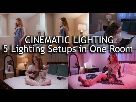
7 Easy Portrait Lighting Setups
Read more: 7 Easy Portrait Lighting Setups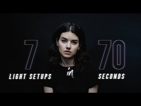
Butterfly
Loop
Rembrandt
Split
Rim
Broad
Short


COLLECTIONS
| Featured AI
| Design And Composition
| Explore posts
POPULAR SEARCHES
unreal | pipeline | virtual production | free | learn | photoshop | 360 | macro | google | nvidia | resolution | open source | hdri | real-time | photography basics | nuke
FEATURED POSTS
-
FFmpeg – examples and convenience lines
-
Web vs Printing or digital RGB vs CMYK
-
Animation/VFX/Game Industry JOB POSTINGS by Chris Mayne
-
NVidia – High-Fidelity 3D Mesh Generation at Scale with Meshtron
-
ComfyDock – The Easiest (Free) Way to Safely Run ComfyUI Sessions in a Boxed Container
-
Blender VideoDepthAI – Turn any video into 3D Animated Scenes
-
QR code logos
-
Top 3D Printing Website Resources
Social Links
DISCLAIMER – Links and images on this website may be protected by the respective owners’ copyright. All data submitted by users through this site shall be treated as freely available to share.
