


COMPOSITION
-
Christopher Butler – Understanding the Eye-Mind Connection – Vision is a mental process
Read more: Christopher Butler – Understanding the Eye-Mind Connection – Vision is a mental processhttps://www.chrbutler.com/understanding-the-eye-mind-connection
The intricate relationship between the eyes and the brain, often termed the eye-mind connection, reveals that vision is predominantly a cognitive process. This understanding has profound implications for fields such as design, where capturing and maintaining attention is paramount. This essay delves into the nuances of visual perception, the brain’s role in interpreting visual data, and how this knowledge can be applied to effective design strategies.
This cognitive aspect of vision is evident in phenomena such as optical illusions, where the brain interprets visual information in a way that contradicts physical reality. These illusions underscore that what we “see” is not merely a direct recording of the external world but a constructed experience shaped by cognitive processes.
Understanding the cognitive nature of vision is crucial for effective design. Designers must consider how the brain processes visual information to create compelling and engaging visuals. This involves several key principles:
- Attention and Engagement
- Visual Hierarchy
- Cognitive Load Management
- Context and Meaning


DESIGN
-
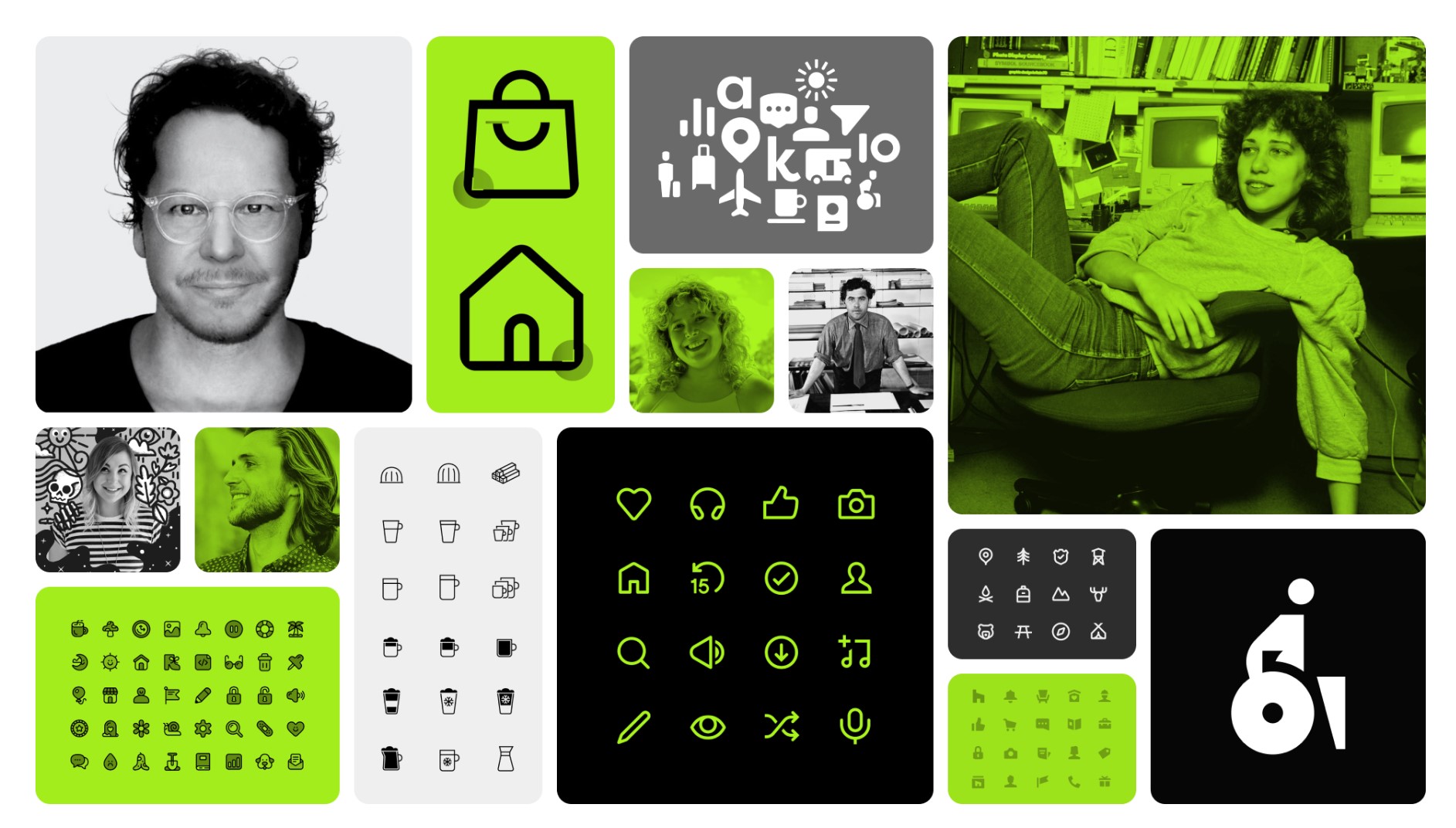
The 7 key elements of brand identity design + 10 corporate identity examples
Read more: The 7 key elements of brand identity design + 10 corporate identity exampleswww.lucidpress.com/blog/the-7-key-elements-of-brand-identity-design
1. Clear brand purpose and positioning
2. Thorough market research
3. Likable brand personality
4. Memorable logo
5. Attractive color palette
6. Professional typography
7. On-brand supporting graphics

-
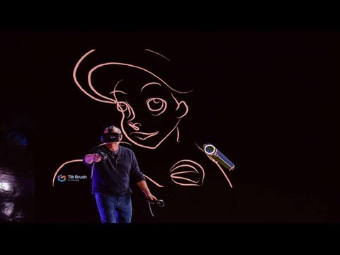
Kristina Kashtanova – “This is how GPT-4 sees and hears itself”
Read more: Kristina Kashtanova – “This is how GPT-4 sees and hears itself”“I used GPT-4 to describe itself. Then I used its description to generate an image, a video based on this image and a soundtrack.
Tools I used: GPT-4, Midjourney, Kaiber AI, Mubert, RunwayML
This is the description I used that GPT-4 had of itself as a prompt to text-to-image, image-to-video, and text-to-music. I put the video and sound together in RunwayML.
GPT-4 described itself as: “Imagine a sleek, metallic sphere with a smooth surface, representing the vast knowledge contained within the model. The sphere emits a soft, pulsating glow that shifts between various colors, symbolizing the dynamic nature of the AI as it processes information and generates responses. The sphere appears to float in a digital environment, surrounded by streams of data and code, reflecting the complex algorithms and computing power behind the AI”


COLOR
-
The Forbidden colors – Red-Green & Blue-Yellow: The Stunning Colors You Can’t See
Read more: The Forbidden colors – Red-Green & Blue-Yellow: The Stunning Colors You Can’t Seewww.livescience.com/17948-red-green-blue-yellow-stunning-colors.html

While the human eye has red, green, and blue-sensing cones, those cones are cross-wired in the retina to produce a luminance channel plus a red-green and a blue-yellow channel, and it’s data in that color space (known technically as “LAB”) that goes to the brain. That’s why we can’t perceive a reddish-green or a yellowish-blue, whereas such colors can be represented in the RGB color space used by digital cameras.
https://en.rockcontent.com/blog/the-use-of-yellow-in-data-design
The back of the retina is covered in light-sensitive neurons known as cone cells and rod cells. There are three types of cone cells, each sensitive to different ranges of light. These ranges overlap, but for convenience the cones are referred to as blue (short-wavelength), green (medium-wavelength), and red (long-wavelength). The rod cells are primarily used in low-light situations, so we’ll ignore those for now.
When light enters the eye and hits the cone cells, the cones get excited and send signals to the brain through the visual cortex. Different wavelengths of light excite different combinations of cones to varying levels, which generates our perception of color. You can see that the red cones are most sensitive to light, and the blue cones are least sensitive. The sensitivity of green and red cones overlaps for most of the visible spectrum.

Here’s how your brain takes the signals of light intensity from the cones and turns it into color information. To see red or green, your brain finds the difference between the levels of excitement in your red and green cones. This is the red-green channel.
To get “brightness,” your brain combines the excitement of your red and green cones. This creates the luminance, or black-white, channel. To see yellow or blue, your brain then finds the difference between this luminance signal and the excitement of your blue cones. This is the yellow-blue channel.
From the calculations made in the brain along those three channels, we get four basic colors: blue, green, yellow, and red. Seeing blue is what you experience when low-wavelength light excites the blue cones more than the green and red.
Seeing green happens when light excites the green cones more than the red cones. Seeing red happens when only the red cones are excited by high-wavelength light.
Here’s where it gets interesting. Seeing yellow is what happens when BOTH the green AND red cones are highly excited near their peak sensitivity. This is the biggest collective excitement that your cones ever have, aside from seeing pure white.
Notice that yellow occurs at peak intensity in the graph to the right. Further, the lens and cornea of the eye happen to block shorter wavelengths, reducing sensitivity to blue and violet light.
-
Photography basics: Lumens vs Candelas (candle) vs Lux vs FootCandle vs Watts vs Irradiance vs Illuminance
Read more: Photography basics: Lumens vs Candelas (candle) vs Lux vs FootCandle vs Watts vs Irradiance vs Illuminancehttps://www.translatorscafe.com/unit-converter/en-US/illumination/1-11/

The power output of a light source is measured using the unit of watts W. This is a direct measure to calculate how much power the light is going to drain from your socket and it is not relatable to the light brightness itself.
The amount of energy emitted from it per second. That energy comes out in a form of photons which we can crudely represent with rays of light coming out of the source. The higher the power the more rays emitted from the source in a unit of time.
Not all energy emitted is visible to the human eye, so we often rely on photometric measurements, which takes in account the sensitivity of human eye to different wavelenghts


Details in the post
(more…) -
Virtual Production volumes study
Read more: Virtual Production volumes studyColor Fidelity in LED Volumes
https://theasc.com/articles/color-fidelity-in-led-volumes
Virtual Production Glossary
https://vpglossary.com/What is Virtual Production – In depth analysis
https://www.leadingledtech.com/what-is-a-led-virtual-production-studio-in-depth-technical-analysis/
A comparison of LED panels for use in Virtual Production:
Findings and recommendations
https://eprints.bournemouth.ac.uk/36826/1/LED_Comparison_White_Paper%281%29.pdf -
Willem Zwarthoed – Aces gamut in VFX production pdf
Read more: Willem Zwarthoed – Aces gamut in VFX production pdfhttps://www.provideocoalition.com/color-management-part-12-introducing-aces/
Local copy:
https://www.slideshare.net/hpduiker/acescg-a-common-color-encoding-for-visual-effects-applications
-
Is a MacBeth Colour Rendition Chart the Safest Way to Calibrate a Camera?
Read more: Is a MacBeth Colour Rendition Chart the Safest Way to Calibrate a Camera?www.colour-science.org/posts/the-colorchecker-considered-mostly-harmless/
“Unless you have all the relevant spectral measurements, a colour rendition chart should not be used to perform colour-correction of camera imagery but only for white balancing and relative exposure adjustments.”
“Using a colour rendition chart for colour-correction might dramatically increase error if the scene light source spectrum is different from the illuminant used to compute the colour rendition chart’s reference values.”
“other factors make using a colour rendition chart unsuitable for camera calibration:
– Uncontrolled geometry of the colour rendition chart with the incident illumination and the camera.
– Unknown sample reflectances and ageing as the colour of the samples vary with time.
– Low samples count.
– Camera noise and flare.
– Etc…“Those issues are well understood in the VFX industry, and when receiving plates, we almost exclusively use colour rendition charts to white balance and perform relative exposure adjustments, i.e. plate neutralisation.”
-
Stefan Ringelschwandtner – LUT Inspector tool
Read more: Stefan Ringelschwandtner – LUT Inspector toolIt lets you load any .cube LUT right in your browser, see the RGB curves, and use a split view on the Granger Test Image to compare the original vs. LUT-applied version in real time — perfect for spotting hue shifts, saturation changes, and contrast tweaks.
https://mononodes.com/lut-inspector/


-
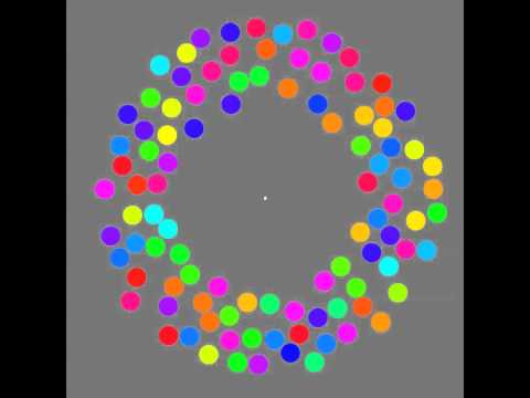
Mysterious animation wins best illusion of 2011 – Motion silencing illusion
Read more: Mysterious animation wins best illusion of 2011 – Motion silencing illusionThe 2011 Best Illusion of the Year uses motion to render color changes invisible, and so reveals a quirk in our visual systems that is new to scientists.
https://en.wikipedia.org/wiki/Motion_silencing_illusion
“It is a really beautiful effect, revealing something about how our visual system works that we didn’t know before,” said Daniel Simons, a professor at the University of Illinois, Champaign-Urbana. Simons studies visual cognition, and did not work on this illusion. Before its creation, scientists didn’t know that motion had this effect on perception, Simons said.
A viewer stares at a speck at the center of a ring of colored dots, which continuously change color. When the ring begins to rotate around the speck, the color changes appear to stop. But this is an illusion. For some reason, the motion causes our visual system to ignore the color changes. (You can, however, see the color changes if you follow the rotating circles with your eyes.)


LIGHTING
-
GretagMacbeth Color Checker Numeric Values and Middle Gray
Read more: GretagMacbeth Color Checker Numeric Values and Middle GrayThe human eye perceives half scene brightness not as the linear 50% of the present energy (linear nature values) but as 18% of the overall brightness. We are biased to perceive more information in the dark and contrast areas. A Macbeth chart helps with calibrating back into a photographic capture into this “human perspective” of the world.
https://en.wikipedia.org/wiki/Middle_gray
In photography, painting, and other visual arts, middle gray or middle grey is a tone that is perceptually about halfway between black and white on a lightness scale in photography and printing, it is typically defined as 18% reflectance in visible light

Light meters, cameras, and pictures are often calibrated using an 18% gray card[4][5][6] or a color reference card such as a ColorChecker. On the assumption that 18% is similar to the average reflectance of a scene, a grey card can be used to estimate the required exposure of the film.
https://en.wikipedia.org/wiki/ColorChecker
(more…) -
Composition – cinematography Cheat Sheet
Read more: Composition – cinematography Cheat Sheet
Where is our eye attracted first? Why?
Size. Focus. Lighting. Color.
Size. Mr. White (Harvey Keitel) on the right.
Focus. He’s one of the two objects in focus.
Lighting. Mr. White is large and in focus and Mr. Pink (Steve Buscemi) is highlighted by
a shaft of light.
Color. Both are black and white but the read on Mr. White’s shirt now really stands out.
(more…)
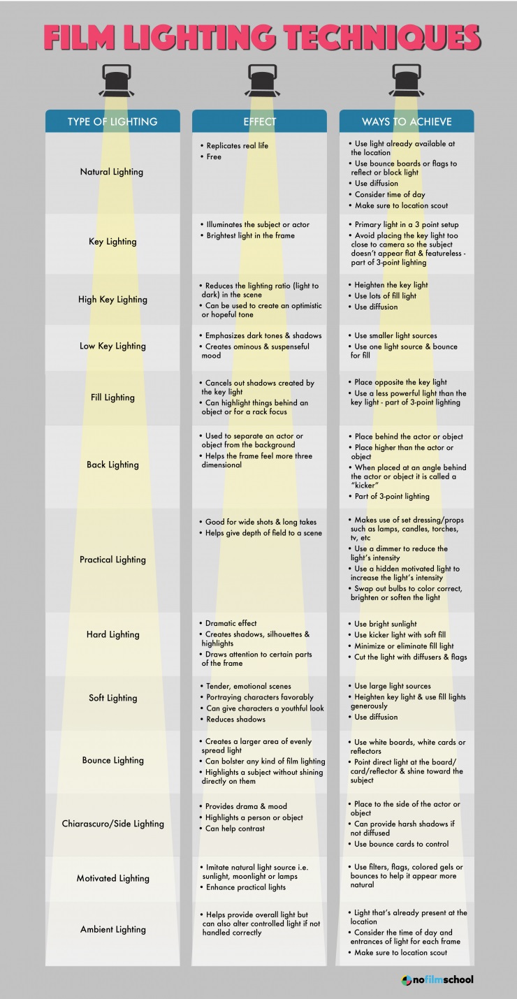
What type of lighting?


COLLECTIONS
| Featured AI
| Design And Composition
| Explore posts
POPULAR SEARCHES
unreal | pipeline | virtual production | free | learn | photoshop | 360 | macro | google | nvidia | resolution | open source | hdri | real-time | photography basics | nuke
FEATURED POSTS
-
PixelSham – Introduction to Python 2022
-
Photography basics: Solid Angle measures
-
Canva bought Affinity – Now Affinity Photo and Affinity Designer are… GONE?!
-
Convert 2D Images or Text to 3D Models
-
How to paint a boardgame miniatures
-
Gamma correction
-
Methods for creating motion blur in Stop motion
-
The Public Domain Is Working Again — No Thanks To Disney
Social Links
DISCLAIMER – Links and images on this website may be protected by the respective owners’ copyright. All data submitted by users through this site shall be treated as freely available to share.
