To measure the contrast ratio you will need a light meter. The process starts with you measuring the main source of light, or the key light.
Get a reading from the brightest area on the face of your subject. Then, measure the area lit by the secondary light, or fill light. To make sense of what you have just measured you have to understand that the information you have just gathered is in F-stops, a measure of light. With each additional F-stop, for example going one stop from f/1.4 to f/2.0, you create a doubling of light. The reverse is also true; moving one stop from f/8.0 to f/5.6 results in a halving of the light.
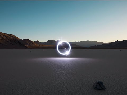
Wu programmed a stick of 200 LED lights to shift in color and shape above the calm landscapes. He captured the mesmerizing movements in-camera, and through a combination of stills, timelapse, and real-time footage, produced four audiovisual works that juxtapose the natural scenery with the artificially produced light and electronic sounds.
Display Referred it is tied to the target hardware, as such it bakes color requirements into every type of media output request.
Scene Referred uses a common unified wide gamut and targeting audience through CDL and DI libraries instead.
So that color information stays untouched and only “transformed” as/when needed.
Sources:
– Victor Perez – Color Management Fundamentals & ACES Workflows in Nuke
– https://z-fx.nl/ColorspACES.pdf – Wicus
In HD we often refer to the range of available colors as a color gamut. Such a color gamut is typically plotted on a two-dimensional diagram, called a CIE chart, as shown in at the top of this blog. Each color is characterized by its x/y coordinates.
Good enough for government work, perhaps. But for HDR, with its higher luminance levels and wider color, the gamut becomes three-dimensional.
For HDR the color gamut therefore becomes a characteristic we now call the color volume. It isn’t easy to show color volume on a two-dimensional medium like the printed page or a computer screen, but one method is shown below. As the luminance becomes higher, the picture eventually turns to white. As it becomes darker, it fades to black. The traditional color gamut shown on the CIE chart is simply a slice through this color volume at a selected luminance level, such as 50%.
Three different color volumes—we still refer to them as color gamuts though their third dimension is important—are currently the most significant. The first is BT.709 (sometimes referred to as Rec.709), the color gamut used for pre-UHD/HDR formats, including standard HD.
The largest is known as BT.2020; it encompasses (roughly) the range of colors visible to the human eye (though ET might find it insufficient!).
Between these two is the color gamut used in digital cinema, known as DCI-P3.
In color technology, color depth also known as bit depth, is either the number of bits used to indicate the color of a single pixel, OR the number of bits used for each color component of a single pixel.
When referring to a pixel, the concept can be defined as bits per pixel (bpp).
When referring to a color component, the concept can be defined as bits per component, bits per channel, bits per color (all three abbreviated bpc), and also bits per pixel component, bits per color channel or bits per sample (bps). Modern standards tend to use bits per component, but historical lower-depth systems used bits per pixel more often.
Color depth is only one aspect of color representation, expressing the precision with which the amount of each primary can be expressed; the other aspect is how broad a range of colors can be expressed (the gamut). The definition of both color precision and gamut is accomplished with a color encoding specification which assigns a digital code value to a location in a color space.
5.10 of this tool includes excellent tools to clean up cr2 and cr3 used on set to support HDRI processing.
Converting raw to AcesCG 32 bit tiffs with metadata.
import math,sys

def Exposure2Intensity(exposure):
    exp = float(exposure)
    result = math.pow(2,exp)
    print(result)

Exposure2Intensity(0)

def Intensity2Exposure(intensity):
    inarg = float(intensity)

    if inarg == 0:
        print("Exposure of zero intensity is undefined.")
        return

    if inarg < 1e-323:
        inarg = max(inarg, 1e-323)
        print("Exposure of negative intensities is undefined. Clamping to a very small value instead (1e-323)")

    result = math.log(inarg, 2)
    print(result)

Intensity2Exposure(0.1)
Why Exposure?
Exposure is a stop value that multiplies the intensity by 2 to the power of the stop. Increasing exposure by 1 results in double the amount of light.
Artists think in “stops.” Doubling or halving brightness is easy math and common in grading and look-dev. Exposure counts doublings in whole stops:
+1 stop = ×2 brightness
−1 stop = ×0.5 brightness
This gives perceptually even controls across both bright and dark values.
Why Intensity?
Intensity is linear. It’s what render engines and compositors expect when:
Summing values
Averaging pixels
Multiplying or filtering pixel data
Use intensity when you need the actual math on pixel/light data.
Formulas (from your Python)
Intensity from exposure: intensity = 2**exposure
Exposure from intensity: exposure = log₂(intensity)
Guardrails:
Intensity must be > 0 to compute exposure.
If intensity = 0 → exposure is undefined.
Clamp tiny values (e.g. 1e−323) before using log₂.
Use Exposure (stops) when…
You want artist-friendly sliders (−5…+5 stops)
Adjusting look-dev or grading in even stops
Matching plates with quick ±1 stop tweaks
Tweening brightness changes smoothly across ranges
Use Intensity (linear) when…
Storing raw pixel/light values
Multiplying textures or lights by a gain
Performing sums, averages, and filters
Feeding values to render engines expecting linear data
Examples
+2 stops → 2**2 = 4.0 (×4)
+1 stop → 2**1 = 2.0 (×2)
0 stop → 2**0 = 1.0 (×1)
−1 stop → 2**(−1) = 0.5 (×0.5)
−2 stops → 2**(−2) = 0.25 (×0.25)
Intensity 0.1 → exposure = log₂(0.1) ≈ −3.32
Rule of thumb
Think in stops (exposure) for controls and matching. Compute in linear (intensity) for rendering and math.
Bella works in spectral space, allowing effects such as BSDF wavelength dependency, diffraction, or atmosphere to be modeled far more accurately than in color space.
Physically-based shading means leaving behind phenomenological models, like the Phong shading model, which are simply built to “look good” subjectively without being based on physics in any real way, and moving to lighting and shading models that are derived from the laws of physics and/or from actual measurements of the real world, and rigorously obey physical constraints such as energy conservation.
For example, in many older rendering systems, shading models included separate controls for specular highlights from point lights and reflection of the environment via a cubemap. You could create a shader with the specular and the reflection set to wildly different values, even though those are both instances of the same physical process. In addition, you could set the specular to any arbitrary brightness, even if it would cause the surface to reflect more energy than it actually received.
In a physically-based system, both the point light specular and the environment reflection would be controlled by the same parameter, and the system would be set up to automatically adjust the brightness of both the specular and diffuse components to maintain overall energy conservation. Moreover you would want to set the specular brightness to a realistic value for the material you’re trying to simulate, based on measurements.
Physically-based lighting or shading includes physically-based BRDFs, which are usually based on microfacet theory, and physically correct light transport, which is based on the rendering equation (although heavily approximated in the case of real-time games).
It also includes the necessary changes in the art process to make use of these features. Switching to a physically-based system can cause some upsets for artists. First of all it requires full HDR lighting with a realistic level of brightness for light sources, the sky, etc. and this can take some getting used to for the lighting artists. It also requires texture/material artists to do some things differently (particularly for specular), and they can be frustrated by the apparent loss of control (e.g. locking together the specular highlight and environment reflection as mentioned above; artists will complain about this). They will need some time and guidance to adapt to the physically-based system.
On the plus side, once artists have adapted and gained trust in the physically-based system, they usually end up liking it better, because there are fewer parameters overall (less work for them to tweak). Also, materials created in one lighting environment generally look fine in other lighting environments too. This is unlike more ad-hoc models, where a set of material parameters might look good during daytime, but it comes out ridiculously glowy at night, or something like that.
Here are some resources to look at for physically-based lighting in games:
SIGGRAPH 2013 Physically Based Shading Course, particularly the background talk by Naty Hoffman at the beginning. You can also check out the previous incarnations of this course for more resources.
And of course, I would be remiss if I didn’t mention Physically-Based Rendering by Pharr and Humphreys, an amazing reference on this whole subject and well worth your time, although it focuses on offline rather than real-time rendering.
In general, when light interacts with matter, a complicated light-matter dynamic occurs. This interaction depends on the physical characteristics of the light as well as the physical composition and characteristics of the matter.
That is, some of the incident light is reflected, some of the light is transmitted, and another portion of the light is absorbed by the medium itself.
A BRDF describes how much light is reflected when light makes contact with a certain material. Similarly, a BTDF (Bi-directional Transmission Distribution Function) describes how much light is transmitted when light makes contact with a certain material
It is difficult to establish exactly how far one should go in elaborating the surface model. A truly complete representation of the reflective behavior of a surface might take into account such phenomena as polarization, scattering, fluorescence, and phosphorescence, all of which might vary with position on the surface. Therefore, the variables in this complete function would be:
incoming and outgoing angle incoming and outgoing wavelength incoming and outgoing polarization (both linear and circular) incoming and outgoing position (which might differ due to subsurface scattering) time delay between the incoming and outgoing light ray
“The Color Rendering Index is a measurement of how faithfully a light source reveals the colors of whatever it illuminates, it describes the ability of a light source to reveal the color of an object, as compared to the color a natural light source would provide. The highest possible CRI is 100. A CRI of 100 generally refers to a perfect black body, like a tungsten light source or the sun. ”
DISCLAIMER – Links and images on this website may be protected by the respective owners’ copyright. All data submitted by users through this site shall be treated as freely available to share.