In color technology, color depth also known as bit depth, is either the number of bits used to indicate the color of a single pixel, OR the number of bits used for each color component of a single pixel.
When referring to a pixel, the concept can be defined as bits per pixel (bpp).
When referring to a color component, the concept can be defined as bits per component, bits per channel, bits per color (all three abbreviated bpc), and also bits per pixel component, bits per color channel or bits per sample (bps). Modern standards tend to use bits per component, but historical lower-depth systems used bits per pixel more often.
Color depth is only one aspect of color representation, expressing the precision with which the amount of each primary can be expressed; the other aspect is how broad a range of colors can be expressed (the gamut). The definition of both color precision and gamut is accomplished with a color encoding specification which assigns a digital code value to a location in a color space.
The Manuka rendering architecture has been designed in the spirit of the classic reyes rendering architecture. In its core, reyes is based on stochastic rasterisation of micropolygons, facilitating depth of field, motion blur, high geometric complexity,and programmable shading.
This is commonly achieved with Monte Carlo path tracing, using a paradigm often called shade-on-hit, in which the renderer alternates tracing rays with running shaders on the various ray hits. The shaders take the role of generating the inputs of the local material structure which is then used bypath sampling logic to evaluate contributions and to inform what further rays to cast through the scene.
Over the years, however, the expectations have risen substantially when it comes to image quality. Computing pictures which are indistinguishable from real footage requires accurate simulation of light transport, which is most often performed using some variant of Monte Carlo path tracing. Unfortunately this paradigm requires random memory accesses to the whole scene and does not lend itself well to a rasterisation approach at all.
Manuka is both a uni-directional and bidirectional path tracer and encompasses multiple importance sampling (MIS). Interestingly, and importantly for production character skin work, it is the first major production renderer to incorporate spectral MIS in the form of a new ‘Hero Spectral Sampling’ technique, which was recently published at Eurographics Symposium on Rendering 2014.
Manuka propose a shade-before-hit paradigm in-stead and minimise I/O strain (and some memory costs) on the system, leveraging locality of reference by running pattern generation shaders before we execute light transport simulation by path sampling, “compressing” any bvh structure as needed, and as such also limiting duplication of source data.
The difference with reyes is that instead of baking colors into the geometry like in Reyes, manuka bakes surface closures. This means that light transport is still calculated with path tracing, but all texture lookups etc. are done up-front and baked into the geometry.
The main drawback with this method is that geometry has to be tessellated to its highest, stable topology before shading can be evaluated properly. As such, the high cost to first pixel. Even a basic 4 vertices square becomes a much more complex model with this approach.
Manuka use the RenderMan Shading Language (rsl) for programmable shading [Pixar Animation Studios 2015], but we do not invoke rsl shaders when intersecting a ray with a surface (often called shade-on-hit). Instead, we pre-tessellate and pre-shade all the input geometry in the front end of the renderer.
This way, we can efficiently order shading computations to sup-port near-optimal texture locality, vectorisation, and parallelism. This system avoids repeated evaluation of shaders at the same surface point, and presents a minimal amount of memory to be accessed during light transport time. An added benefit is that the acceleration structure for ray tracing (abounding volume hierarchy, bvh) is built once on the final tessellated geometry, which allows us to ray trace more efficiently than multi-level bvhs and avoids costly caching of on-demand tessellated micropolygons and the associated scheduling issues.
For the shading reasons above, in terms of AOVs, the studio approach is to succeed at combining complex shading with ray paths in the render rather than pass a multi-pass render to compositing.
For the Spectral Rendering component. The light transport stage is fully spectral, using a continuously sampled wavelength which is traced with each path and used to apply the spectral camera sensitivity of the sensor. This allows for faithfully support any degree of observer metamerism as the camera footage they are intended to match as well as complex materials which require wavelength dependent phenomena such as diffraction, dispersion, interference, iridescence, or chromatic extinction and Rayleigh scattering in participating media.
As opposed to the original reyes paper, we use bilinear interpolation of these bsdf inputs later when evaluating bsdfs per pathv ertex during light transport4. This improves temporal stability of geometry which moves very slowly with respect to the pixel raster
In terms of the pipeline, everything rendered at Weta was already completely interwoven with their deep data pipeline. Manuka very much was written with deep data in mind. Here, Manuka not so much extends the deep capabilities, rather it fully matches the already extremely complex and powerful setup Weta Digital already enjoy with RenderMan. For example, an ape in a scene can be selected, its ID is available and a NUKE artist can then paint in 3D say a hand and part of the way up the neutral posed ape.
We called our system Manuka, as a respectful nod to reyes: we had heard a story froma former ILM employee about how reyes got its name from how fond the early Pixar people were of their lunches at Point Reyes, and decided to name our system after our surrounding natural environment, too. Manuka is a kind of tea tree very common in New Zealand which has very many very small leaves, in analogy to micropolygons ina tree structure for ray tracing. It also happens to be the case that Weta Digital’s main site is on Manuka Street.
Color Temperature of a light source describes the spectrum of light which is radiated from a theoretical “blackbody” (an ideal physical body that absorbs all radiation and incident light – neither reflecting it nor allowing it to pass through) with a given surface temperature.
Or. Most simply it is a method of describing the color characteristics of light through a numerical value that corresponds to the color emitted by a light source, measured in degrees of Kelvin (K) on a scale from 1,000 to 10,000.
More accurately. The color temperature of a light source is the temperature of an ideal backbody that radiates light of comparable hue to that of the light source.
Note: In Foundry’s Nuke, the software will map 18% gray to whatever your center f/stop is set to in the viewer settings (f/8 by default… change that to EV by following the instructions below).
You can experiment with this by attaching an Exposure node to a Constant set to 0.18, setting your viewer read-out to Spotmeter, and adjusting the stops in the node up and down. You will see that a full stop up or down will give you the respective next value on the aperture scale (f8, f11, f16 etc.).
One stop doubles or halves the amount or light that hits the filmback/ccd, so everything works in powers of 2.
So starting with 0.18 in your constant, you will see that raising it by a stop will give you .36 as a floating point number (in linear space), while your f/stop will be f/11 and so on.
If you set your center stop to 0 (see below) you will get a relative readout in EVs, where EV 0 again equals 18% constant gray.
In other words. Setting the center f-stop to 0 means that in a neutral plate, the middle gray in the macbeth chart will equal to exposure value 0. EV 0 corresponds to an exposure time of 1 sec and an aperture of f/1.0.
This will set the sun usually around EV12-17 and the sky EV1-4 , depending on cloud coverage.
To switch Foundry’s Nuke’s SpotMeter to return the EV of an image, click on the main viewport, and then press s, this opens the viewer’s properties. Now set the center f-stop to 0 in there. And the SpotMeter in the viewport will change from aperture and fstops to EV.
Black-body radiation is the type of electromagnetic radiation within or surrounding a body in thermodynamic equilibrium with its environment, or emitted by a black body (an opaque and non-reflective body) held at constant, uniform temperature. The radiation has a specific spectrum and intensity that depends only on the temperature of the body.
A black-body at room temperature appears black, as most of the energy it radiates is infra-red and cannot be perceived by the human eye. At higher temperatures, black bodies glow with increasing intensity and colors that range from dull red to blindingly brilliant blue-white as the temperature increases.
OpenColorIO (OCIO) is a new open source project from Sony Imageworks.
Based on development started in 2003, OCIO enables color transforms and image display to be handled in a consistent manner across multiple graphics applications. Unlike other color management solutions, OCIO is geared towards motion-picture post production, with an emphasis on visual effects and animation color pipelines.
import math,sys

def Exposure2Intensity(exposure):
    exp = float(exposure)
    result = math.pow(2,exp)
    print(result)

Exposure2Intensity(0)

def Intensity2Exposure(intensity):
    inarg = float(intensity)

    if inarg == 0:
        print("Exposure of zero intensity is undefined.")
        return

    if inarg < 1e-323:
        inarg = max(inarg, 1e-323)
        print("Exposure of negative intensities is undefined. Clamping to a very small value instead (1e-323)")

    result = math.log(inarg, 2)
    print(result)

Intensity2Exposure(0.1)
Why Exposure?
Exposure is a stop value that multiplies the intensity by 2 to the power of the stop. Increasing exposure by 1 results in double the amount of light.
Artists think in “stops.” Doubling or halving brightness is easy math and common in grading and look-dev. Exposure counts doublings in whole stops:
+1 stop = ×2 brightness
−1 stop = ×0.5 brightness
This gives perceptually even controls across both bright and dark values.
Why Intensity?
Intensity is linear. It’s what render engines and compositors expect when:
Summing values
Averaging pixels
Multiplying or filtering pixel data
Use intensity when you need the actual math on pixel/light data.
Formulas (from your Python)
Intensity from exposure: intensity = 2**exposure
Exposure from intensity: exposure = log₂(intensity)
Guardrails:
Intensity must be > 0 to compute exposure.
If intensity = 0 → exposure is undefined.
Clamp tiny values (e.g. 1e−323) before using log₂.
Use Exposure (stops) when…
You want artist-friendly sliders (−5…+5 stops)
Adjusting look-dev or grading in even stops
Matching plates with quick ±1 stop tweaks
Tweening brightness changes smoothly across ranges
Use Intensity (linear) when…
Storing raw pixel/light values
Multiplying textures or lights by a gain
Performing sums, averages, and filters
Feeding values to render engines expecting linear data
Examples
+2 stops → 2**2 = 4.0 (×4)
+1 stop → 2**1 = 2.0 (×2)
0 stop → 2**0 = 1.0 (×1)
−1 stop → 2**(−1) = 0.5 (×0.5)
−2 stops → 2**(−2) = 0.25 (×0.25)
Intensity 0.1 → exposure = log₂(0.1) ≈ −3.32
Rule of thumb
Think in stops (exposure) for controls and matching. Compute in linear (intensity) for rendering and math.
The goals of lighting in 3D computer graphics are more or less the same as those of real world lighting.
Lighting serves a basic function of bringing out, or pushing back the shapes of objects visible from the camera’s view.
It gives a two-dimensional image on the monitor an illusion of the third dimension-depth.
But it does not just stop there. It gives an image its personality, its character. A scene lit in different ways can give a feeling of happiness, of sorrow, of fear etc., and it can do so in dramatic or subtle ways. Along with personality and character, lighting fills a scene with emotion that is directly transmitted to the viewer.
Trying to simulate a real environment in an artificial one can be a daunting task. But even if you make your 3D rendering look absolutely photo-realistic, it doesn’t guarantee that the image carries enough emotion to elicit a “wow” from the people viewing it.
Making 3D renderings photo-realistic can be hard. Putting deep emotions in them can be even harder. However, if you plan out your lighting strategy for the mood and emotion that you want your rendering to express, you make the process easier for yourself.
Each light source can be broken down in to 4 distinct components and analyzed accordingly.
· Intensity
· Direction
· Color
· Size
The overall thrust of this writing is to produce photo-realistic images by applying good lighting techniques.
In general, when light interacts with matter, a complicated light-matter dynamic occurs. This interaction depends on the physical characteristics of the light as well as the physical composition and characteristics of the matter.
That is, some of the incident light is reflected, some of the light is transmitted, and another portion of the light is absorbed by the medium itself.
A BRDF describes how much light is reflected when light makes contact with a certain material. Similarly, a BTDF (Bi-directional Transmission Distribution Function) describes how much light is transmitted when light makes contact with a certain material
It is difficult to establish exactly how far one should go in elaborating the surface model. A truly complete representation of the reflective behavior of a surface might take into account such phenomena as polarization, scattering, fluorescence, and phosphorescence, all of which might vary with position on the surface. Therefore, the variables in this complete function would be:
incoming and outgoing angle incoming and outgoing wavelength incoming and outgoing polarization (both linear and circular) incoming and outgoing position (which might differ due to subsurface scattering) time delay between the incoming and outgoing light ray
Basically, gamma is the relationship between the brightness of a pixel as it appears on the screen, and the numerical value of that pixel. Generally Gamma is just about defining relationships.
Three main types: – Image Gamma encoded in images – Display Gammas encoded in hardware and/or viewing time – System or Viewing Gamma which is the net effect of all gammas when you look back at a final image. In theory this should flatten back to 1.0 gamma.
DISCLAIMER – Links and images on this website may be protected by the respective owners’ copyright. All data submitted by users through this site shall be treated as freely available to share.