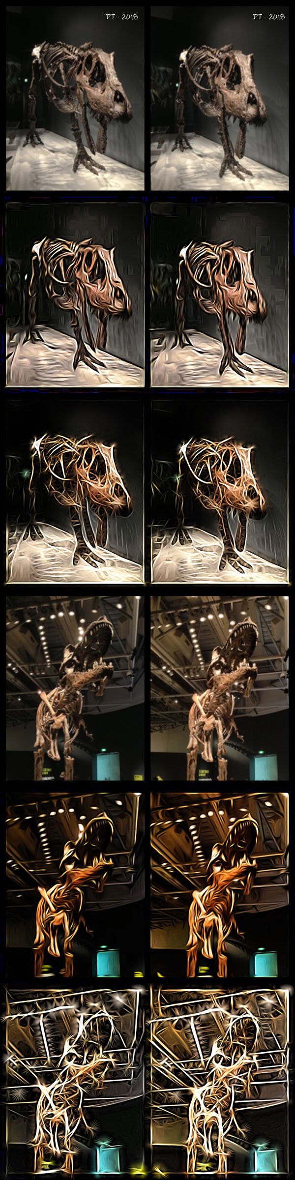
slowmoVideo is an OpenSource program that creates slow-motion videos from your footage.
Slow motion cinematography is the result of playing back frames for a longer duration than they were exposed. For example, if you expose 240 frames of film in one second, then play them back at 24 fps, the resulting movie is 10 times longer (slower) than the original filmed event….
Film cameras are relatively simple mechanical devices that allow you to crank up the speed to whatever rate the shutter and pull-down mechanism allow. Some film cameras can operate at 2,500 fps or higher (although film shot in these cameras often needs some readjustment in postproduction). Video, on the other hand, is always captured, recorded, and played back at a fixed rate, with a current limit around 60fps. This makes extreme slow motion effects harder to achieve (and less elegant) on video, because slowing down the video results in each frame held still on the screen for a long time, whereas with high-frame-rate film there are plenty of frames to fill the longer durations of time. On video, the slow motion effect is more like a slide show than smooth, continuous motion.
One obvious solution is to shoot film at high speed, then transfer it to video (a case where film still has a clear advantage, sorry George). Another possibility is to cross dissolve or blur from one frame to the next. This adds a smooth transition from one still frame to the next. The blur reduces the sharpness of the image, and compared to slowing down images shot at a high frame rate, this is somewhat of a cheat. However, there isn’t much you can do about it until video can be recorded at much higher rates. Of course, many film cameras can’t shoot at high frame rates either, so the whole super-slow-motion endeavor is somewhat specialized no matter what medium you are using. (There are some high speed digital cameras available now that allow you to capture lots of digital frames directly to your computer, so technology is starting to catch up with film. However, this feature isn’t going to appear in consumer camcorders any time soon.)
While the human eye has red, green, and blue-sensing cones, those cones are cross-wired in the retina to produce a luminance channel plus a red-green and a blue-yellow channel, and it’s data in that color space (known technically as “LAB”) that goes to the brain. That’s why we can’t perceive a reddish-green or a yellowish-blue, whereas such colors can be represented in the RGB color space used by digital cameras.
The back of the retina is covered in light-sensitive neurons known as cone cells and rod cells. There are three types of cone cells, each sensitive to different ranges of light. These ranges overlap, but for convenience the cones are referred to as blue (short-wavelength), green (medium-wavelength), and red (long-wavelength). The rod cells are primarily used in low-light situations, so we’ll ignore those for now.
When light enters the eye and hits the cone cells, the cones get excited and send signals to the brain through the visual cortex. Different wavelengths of light excite different combinations of cones to varying levels, which generates our perception of color. You can see that the red cones are most sensitive to light, and the blue cones are least sensitive. The sensitivity of green and red cones overlaps for most of the visible spectrum.
Here’s how your brain takes the signals of light intensity from the cones and turns it into color information. To see red or green, your brain finds the difference between the levels of excitement in your red and green cones. This is the red-green channel.
To get “brightness,” your brain combines the excitement of your red and green cones. This creates the luminance, or black-white, channel. To see yellow or blue, your brain then finds the difference between this luminance signal and the excitement of your blue cones. This is the yellow-blue channel.
From the calculations made in the brain along those three channels, we get four basic colors: blue, green, yellow, and red. Seeing blue is what you experience when low-wavelength light excites the blue cones more than the green and red.
Seeing green happens when light excites the green cones more than the red cones. Seeing red happens when only the red cones are excited by high-wavelength light.
Here’s where it gets interesting. Seeing yellow is what happens when BOTH the green AND red cones are highly excited near their peak sensitivity. This is the biggest collective excitement that your cones ever have, aside from seeing pure white.
Notice that yellow occurs at peak intensity in the graph to the right. Further, the lens and cornea of the eye happen to block shorter wavelengths, reducing sensitivity to blue and violet light.
A LUT (Lookup Table) is essentially the modifier between two images, the original image and the displayed image, based on a mathematical formula. Basically conversion matrices of different complexities. There are different types of LUTS – viewing, transform, calibration, 1D and 3D.
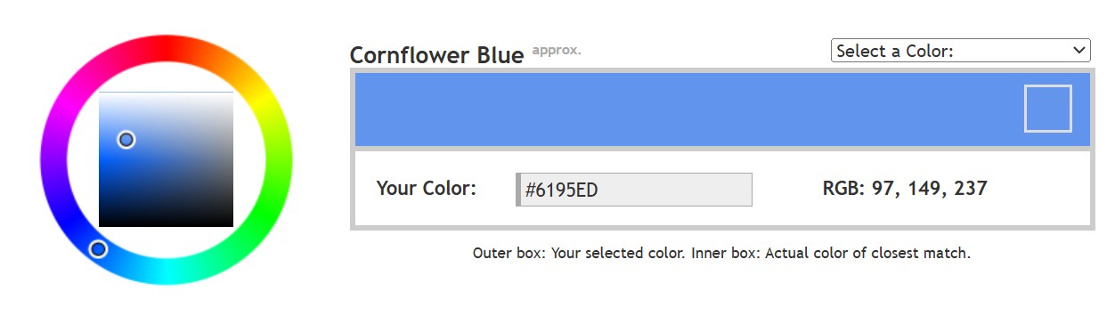
In color technology, color depth also known as bit depth, is either the number of bits used to indicate the color of a single pixel, OR the number of bits used for each color component of a single pixel.
When referring to a pixel, the concept can be defined as bits per pixel (bpp).
When referring to a color component, the concept can be defined as bits per component, bits per channel, bits per color (all three abbreviated bpc), and also bits per pixel component, bits per color channel or bits per sample (bps). Modern standards tend to use bits per component, but historical lower-depth systems used bits per pixel more often.
Color depth is only one aspect of color representation, expressing the precision with which the amount of each primary can be expressed; the other aspect is how broad a range of colors can be expressed (the gamut). The definition of both color precision and gamut is accomplished with a color encoding specification which assigns a digital code value to a location in a color space.
This paper presents an introduction to the color pipelines behind modern feature-film visual-effects and animation.
Authored by Jeremy Selan, and reviewed by the members of the VES Technology Committee including Rob Bredow, Dan Candela, Nick Cannon, Paul Debevec, Ray Feeney, Andy Hendrickson, Gautham Krishnamurti, Sam Richards, Jordan Soles, and Sebastian Sylwan.
“a simple yet effective technique to estimate lighting in a single input image. Current techniques rely heavily on HDR panorama datasets to train neural networks to regress an input with limited field-of-view to a full environment map. However, these approaches often struggle with real-world, uncontrolled settings due to the limited diversity and size of their datasets. To address this problem, we leverage diffusion models trained on billions of standard images to render a chrome ball into the input image. Despite its simplicity, this task remains challenging: the diffusion models often insert incorrect or inconsistent objects and cannot readily generate images in HDR format. Our research uncovers a surprising relationship between the appearance of chrome balls and the initial diffusion noise map, which we utilize to consistently generate high-quality chrome balls. We further fine-tune an LDR difusion model (Stable Diffusion XL) with LoRA, enabling it to perform exposure bracketing for HDR light estimation. Our method produces convincing light estimates across diverse settings and demonstrates superior generalization to in-the-wild scenarios.”
The trigger phrase is “equirectangular 360 degree panorama”. I would avoid saying “spherical projection” since that tends to result in non-equirectangular spherical images.
Image resolution should always be a 2:1 aspect ratio. 1024 x 512 or 1408 x 704 work quite well and were used in the training data. 2048 x 1024 also works.
I suggest using a weight of 0.5 – 1.5. If you are having issues with the image generating too flat instead of having the necessary spherical distortion, try increasing the weight above 1, though this could negatively impact small details of the image. For Flux guidance, I recommend a value of about 2.5 for realistic scenes.
Note. The Median Cut algorithm is typically used for color quantization, which involves reducing the number of colors in an image while preserving its visual quality. It doesn’t directly provide a way to identify the brightest areas in an image. However, if you’re interested in identifying the brightest areas, you might want to look into other methods like thresholding, histogram analysis, or edge detection, through openCV for example.
DISCLAIMER – Links and images on this website may be protected by the respective owners’ copyright. All data submitted by users through this site shall be treated as freely available to share.