


COMPOSITION
-
Cinematographers Blueprint 300dpi poster
Read more: Cinematographers Blueprint 300dpi posterThe 300dpi digital poster is now available to all PixelSham.com subscribers.

If you have already subscribed and wish a copy, please send me a note through the contact page.
-
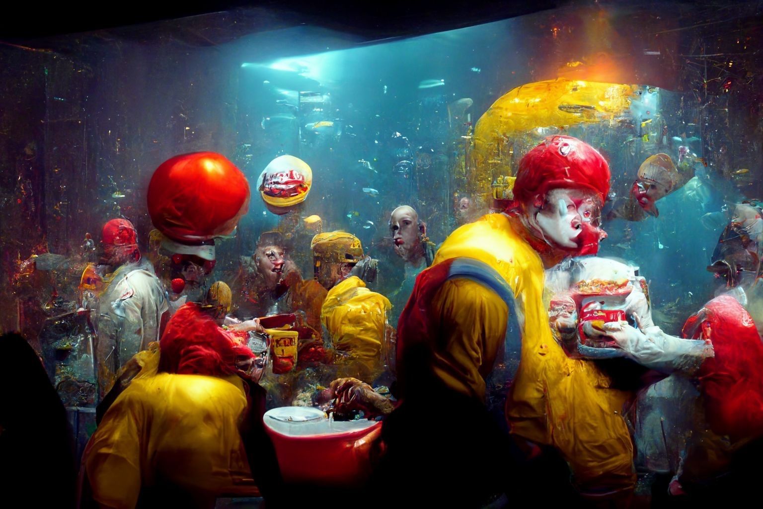
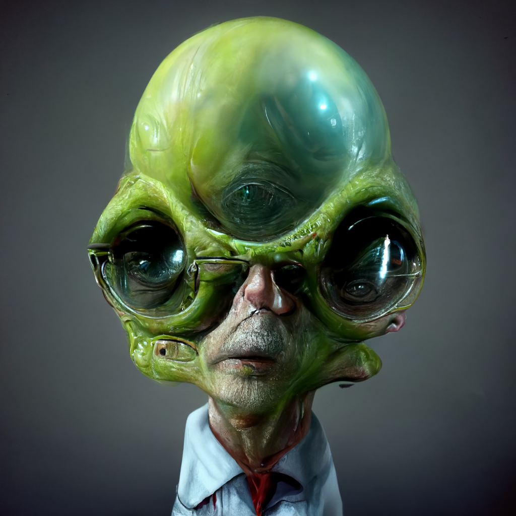
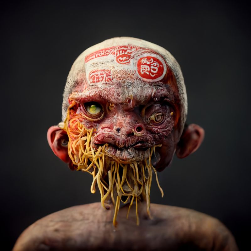
HuggingFace ai-comic-factory – a FREE AI Comic Book Creator
Read more: HuggingFace ai-comic-factory – a FREE AI Comic Book Creatorhttps://huggingface.co/spaces/jbilcke-hf/ai-comic-factory

this is the epic story of a group of talented digital artists trying to overcame daily technical challenges to achieve incredibly photorealistic projects of monsters and aliens


DESIGN
-
Turn Yourself Into an Action Figure Using ChatGPT
Read more: Turn Yourself Into an Action Figure Using ChatGPT
ChatGPT Action Figure Prompts:
Create an action figure from the photo. It must be visualised in a realistic way. There should be accessories next to the figure like a UX designer have, Macbook Pro, a camera, drawing tablet, headset etc. Add a hole to the top of the box in the action figure. Also write the text “UX Mate” and below it “Keep Learning! Keep Designing
Use this image to create a picture of a action figure toy of a construction worker in a blister package from head to toe with accessories including a hammer, a staple gun and a ladder. The package should read “Kirk The Handy Man”
Create a realistic image of a toy action figure box. The box should be designed in a toy-equipment/action-figure style, with a cut-out window at the top like classic action figure packaging. The main color of the box and moleskine notebook should match the color of my jacket (referenced visually). Add colorful Mexican skull decorations across the box for a vibrant and artistic flair. Inside the box, include a “Your name” action figure, posed heroically. Next to the figure, arrange the following “equipment” in a stylized layout: • item 1 • item 2 … On the box, write: “Your name” (bold title font) Underneath: “Your role or anything else” The entire scene should look like a real product mockup, highly realistic, lit like a studio product photo. On the box, write: “Your name” (bold title font) Underneath: “Your role or description” The entire scene should look like a real product mockup, highly realistic, lit like a studio product photo. Prompt on Kling AI The figure steps out of its toy packaging and begins walking forward. As he continues to walk, the camera gradually zooms out in sync with his movement.
“Create image. Create a toy of the person in the photo. Let it be an action figure. Next to the figure, there should be the toy’s equipment, each in its individual blisters. 1) a book called “Tecnoforma”. 2) A 3-headed dog with a tag that says “Troika” and a bone at its feet with word “austerity” written on it. 3) a three-headed Hydra with with a tag called “Geringonça”. 4) a book titled “D. Sebastião”. Don’t repeat the equipment under any circumstance. The card holding the blister should be strong orange. Also, on top of the box, write ‘Pedro Passos Coelho’ and underneath it, ‘PSD action figure’. The figure and equipment must all be inside blisters. Visualize this in a realistic way.”


-
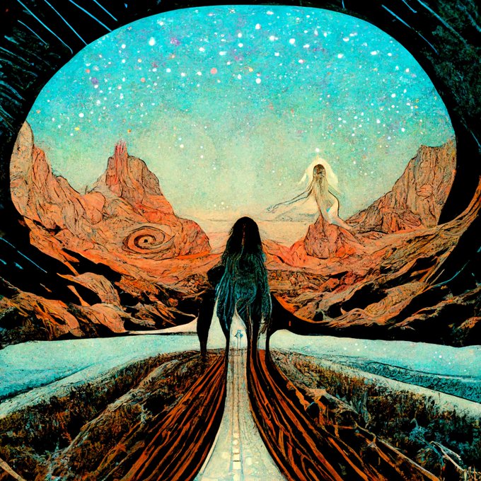
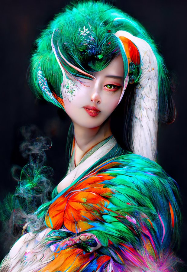
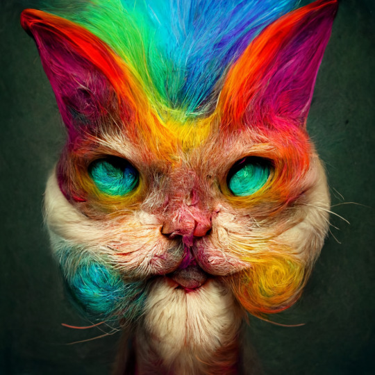
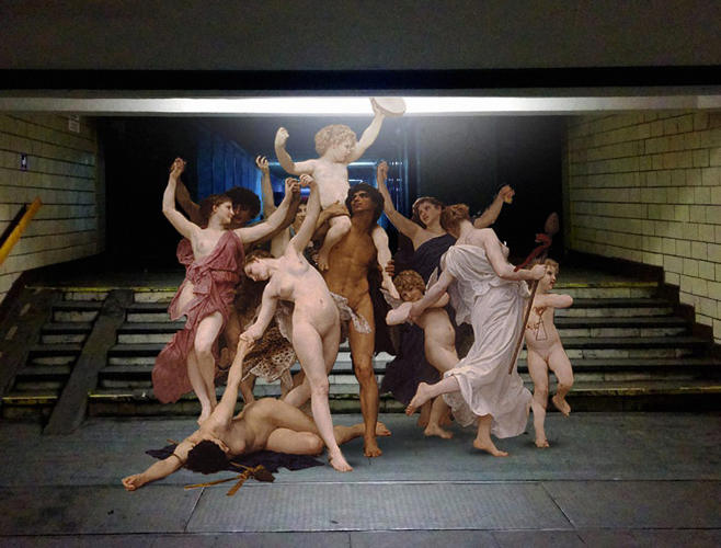
AI MidJourney – creating images with AI
Read more: AI MidJourney – creating images with AIhttps://www.deviantart.com/tag/midjourney
https://boingboing.net/2022/03/24/midjourney-sharpens-style-of-ai-art.html
https://www.resetera.com/threads/midjourney-is-lighting-up-the-ai-generated-art-community.586463/
https://www.artstation.com/artwork/G8Lead
Images courtesy of Midjourney’s users


COLOR
-
Capturing textures albedo
Read more: Capturing textures albedoBuilding a Portable PBR Texture Scanner by Stephane Lb
http://rtgfx.com/pbr-texture-scanner/

How To Split Specular And Diffuse In Real Images, by John Hable
http://filmicworlds.com/blog/how-to-split-specular-and-diffuse-in-real-images/Capturing albedo using a Spectralon
https://www.activision.com/cdn/research/Real_World_Measurements_for_Call_of_Duty_Advanced_Warfare.pdfReal_World_Measurements_for_Call_of_Duty_Advanced_Warfare.pdf
Spectralon is a teflon-based pressed powderthat comes closest to being a pure Lambertian diffuse material that reflects 100% of all light. If we take an HDR photograph of the Spectralon alongside the material to be measured, we can derive thediffuse albedo of that material.

The process to capture diffuse reflectance is very similar to the one outlined by Hable.
1. We put a linear polarizing filter in front of the camera lens and a second linear polarizing filterin front of a modeling light or a flash such that the two filters are oriented perpendicular to eachother, i.e. cross polarized.
2. We place Spectralon close to and parallel with the material we are capturing and take brack-eted shots of the setup7. Typically, we’ll take nine photographs, from -4EV to +4EV in 1EVincrements.
3. We convert the bracketed shots to a linear HDR image. We found that many HDR packagesdo not produce an HDR image in which the pixel values are linear. PTGui is an example of apackage which does generate a linear HDR image. At this point, because of the cross polarization,the image is one of surface diffuse response.
4. We open the file in Photoshop and normalize the image by color picking the Spectralon, filling anew layer with that color and setting that layer to “Divide”. This sets the Spectralon to 1 in theimage. All other color values are relative to this so we can consider them as diffuse albedo.
-
HDR and Color
Read more: HDR and Colorhttps://www.soundandvision.com/content/nits-and-bits-hdr-and-color
In HD we often refer to the range of available colors as a color gamut. Such a color gamut is typically plotted on a two-dimensional diagram, called a CIE chart, as shown in at the top of this blog. Each color is characterized by its x/y coordinates.

Good enough for government work, perhaps. But for HDR, with its higher luminance levels and wider color, the gamut becomes three-dimensional.

For HDR the color gamut therefore becomes a characteristic we now call the color volume. It isn’t easy to show color volume on a two-dimensional medium like the printed page or a computer screen, but one method is shown below. As the luminance becomes higher, the picture eventually turns to white. As it becomes darker, it fades to black. The traditional color gamut shown on the CIE chart is simply a slice through this color volume at a selected luminance level, such as 50%.
Three different color volumes—we still refer to them as color gamuts though their third dimension is important—are currently the most significant. The first is BT.709 (sometimes referred to as Rec.709), the color gamut used for pre-UHD/HDR formats, including standard HD.
The largest is known as BT.2020; it encompasses (roughly) the range of colors visible to the human eye (though ET might find it insufficient!).
Between these two is the color gamut used in digital cinema, known as DCI-P3.

sRGB

D65

-
Photography basics: Why Use a (MacBeth) Color Chart?
Read more: Photography basics: Why Use a (MacBeth) Color Chart?Start here: https://www.pixelsham.com/2013/05/09/gretagmacbeth-color-checker-numeric-values/
https://www.studiobinder.com/blog/what-is-a-color-checker-tool/


In LightRoom

in Final Cut

in Nuke
Note: In Foundry’s Nuke, the software will map 18% gray to whatever your center f/stop is set to in the viewer settings (f/8 by default… change that to EV by following the instructions below).
You can experiment with this by attaching an Exposure node to a Constant set to 0.18, setting your viewer read-out to Spotmeter, and adjusting the stops in the node up and down. You will see that a full stop up or down will give you the respective next value on the aperture scale (f8, f11, f16 etc.).One stop doubles or halves the amount or light that hits the filmback/ccd, so everything works in powers of 2.
So starting with 0.18 in your constant, you will see that raising it by a stop will give you .36 as a floating point number (in linear space), while your f/stop will be f/11 and so on.If you set your center stop to 0 (see below) you will get a relative readout in EVs, where EV 0 again equals 18% constant gray.

In other words. Setting the center f-stop to 0 means that in a neutral plate, the middle gray in the macbeth chart will equal to exposure value 0. EV 0 corresponds to an exposure time of 1 sec and an aperture of f/1.0.
This will set the sun usually around EV12-17 and the sky EV1-4 , depending on cloud coverage.
To switch Foundry’s Nuke’s SpotMeter to return the EV of an image, click on the main viewport, and then press s, this opens the viewer’s properties. Now set the center f-stop to 0 in there. And the SpotMeter in the viewport will change from aperture and fstops to EV.
-
Scientists claim to have discovered ‘new colour’ no one has seen before: Olo
Read more: Scientists claim to have discovered ‘new colour’ no one has seen before: Olohttps://www.bbc.com/news/articles/clyq0n3em41o
By stimulating specific cells in the retina, the participants claim to have witnessed a blue-green colour that scientists have called “olo”, but some experts have said the existence of a new colour is “open to argument”.
The findings, published in the journal Science Advances on Friday, have been described by the study’s co-author, Prof Ren Ng from the University of California, as “remarkable”.

(A) System inputs. (i) Retina map of 103 cone cells preclassified by spectral type (7). (ii) Target visual percept (here, a video of a child, see movie S1 at 1:04). (iii) Infrared cellular-scale imaging of the retina with 60-frames-per-second rolling shutter. Fixational eye movement is visible over the three frames shown.
(B) System outputs. (iv) Real-time per-cone target activation levels to reproduce the target percept, computed by: extracting eye motion from the input video relative to the retina map; identifying the spectral type of every cone in the field of view; computing the per-cone activation the target percept would have produced. (v) Intensities of visible-wavelength 488-nm laser microdoses at each cone required to achieve its target activation level.
(C) Infrared imaging and visible-wavelength stimulation are physically accomplished in a raster scan across the retinal region using AOSLO. By modulating the visible-wavelength beam’s intensity, the laser microdoses shown in (v) are delivered. Drawing adapted with permission [Harmening and Sincich (54)].
(D) Examples of target percepts with corresponding cone activations and laser microdoses, ranging from colored squares to complex imagery. Teal-striped regions represent the color “olo” of stimulating only M cones.
-
Thomas Mansencal – Colour Science for Python
Read more: Thomas Mansencal – Colour Science for Pythonhttps://thomasmansencal.substack.com/p/colour-science-for-python
https://www.colour-science.org/
Colour is an open-source Python package providing a comprehensive number of algorithms and datasets for colour science. It is freely available under the BSD-3-Clause terms.

-
PTGui 13 beta adds control through a Patch Editor
Read more: PTGui 13 beta adds control through a Patch EditorAdditions:
- Patch Editor (PTGui Pro)
- DNG output
- Improved RAW / DNG handling
- JPEG 2000 support
- Performance improvements

-
GretagMacbeth Color Checker Numeric Values and Middle Gray
Read more: GretagMacbeth Color Checker Numeric Values and Middle GrayThe human eye perceives half scene brightness not as the linear 50% of the present energy (linear nature values) but as 18% of the overall brightness. We are biased to perceive more information in the dark and contrast areas. A Macbeth chart helps with calibrating back into a photographic capture into this “human perspective” of the world.
https://en.wikipedia.org/wiki/Middle_gray
In photography, painting, and other visual arts, middle gray or middle grey is a tone that is perceptually about halfway between black and white on a lightness scale in photography and printing, it is typically defined as 18% reflectance in visible light

Light meters, cameras, and pictures are often calibrated using an 18% gray card[4][5][6] or a color reference card such as a ColorChecker. On the assumption that 18% is similar to the average reflectance of a scene, a grey card can be used to estimate the required exposure of the film.
https://en.wikipedia.org/wiki/ColorChecker
(more…) -
Björn Ottosson – OKHSV and OKHSL – Two new color spaces for color picking
Read more: Björn Ottosson – OKHSV and OKHSL – Two new color spaces for color pickinghttps://bottosson.github.io/misc/colorpicker
https://bottosson.github.io/posts/colorpicker/
https://www.smashingmagazine.com/2024/10/interview-bjorn-ottosson-creator-oklab-color-space/
One problem with sRGB is that in a gradient between blue and white, it becomes a bit purple in the middle of the transition. That’s because sRGB really isn’t created to mimic how the eye sees colors; rather, it is based on how CRT monitors work. That means it works with certain frequencies of red, green, and blue, and also the non-linear coding called gamma. It’s a miracle it works as well as it does, but it’s not connected to color perception. When using those tools, you sometimes get surprising results, like purple in the gradient.

There were also attempts to create simple models matching human perception based on XYZ, but as it turned out, it’s not possible to model all color vision that way. Perception of color is incredibly complex and depends, among other things, on whether it is dark or light in the room and the background color it is against. When you look at a photograph, it also depends on what you think the color of the light source is. The dress is a typical example of color vision being very context-dependent. It is almost impossible to model this perfectly.
I based Oklab on two other color spaces, CIECAM16 and IPT. I used the lightness and saturation prediction from CIECAM16, which is a color appearance model, as a target. I actually wanted to use the datasets used to create CIECAM16, but I couldn’t find them.
IPT was designed to have better hue uniformity. In experiments, they asked people to match light and dark colors, saturated and unsaturated colors, which resulted in a dataset for which colors, subjectively, have the same hue. IPT has a few other issues but is the basis for hue in Oklab.
In the Munsell color system, colors are described with three parameters, designed to match the perceived appearance of colors: Hue, Chroma and Value. The parameters are designed to be independent and each have a uniform scale. This results in a color solid with an irregular shape. The parameters are designed to be independent and each have a uniform scale. This results in a color solid with an irregular shape. Modern color spaces and models, such as CIELAB, Cam16 and Björn Ottosson own Oklab, are very similar in their construction.

By far the most used color spaces today for color picking are HSL and HSV, two representations introduced in the classic 1978 paper “Color Spaces for Computer Graphics”. HSL and HSV designed to roughly correlate with perceptual color properties while being very simple and cheap to compute.
Today HSL and HSV are most commonly used together with the sRGB color space.

One of the main advantages of HSL and HSV over the different Lab color spaces is that they map the sRGB gamut to a cylinder. This makes them easy to use since all parameters can be changed independently, without the risk of creating colors outside of the target gamut.

The main drawback on the other hand is that their properties don’t match human perception particularly well.
Reconciling these conflicting goals perfectly isn’t possible, but given that HSV and HSL don’t use anything derived from experiments relating to human perception, creating something that makes a better tradeoff does not seem unreasonable.
With this new lightness estimate, we are ready to look into the construction of Okhsv and Okhsl.


LIGHTING
-
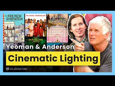
studiobinder.com – What is Tenebrism and Hard Lighting — The Art of Light and Shadow and chiaroscuro Explained
Read more: studiobinder.com – What is Tenebrism and Hard Lighting — The Art of Light and Shadow and chiaroscuro Explainedhttps://www.studiobinder.com/blog/what-is-tenebrism-art-definition/
https://www.studiobinder.com/blog/what-is-hard-light-photography/


-
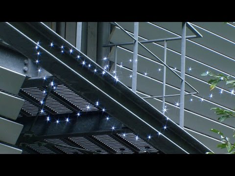
Tracing Spherical harmonics and how Weta used them in production
Read more: Tracing Spherical harmonics and how Weta used them in productionA way to approximate complex lighting in ultra realistic renders.
All SH lighting techniques involve replacing parts of standard lighting equations with spherical functions that have been projected into frequency space using the spherical harmonics as a basis.
http://www.cs.columbia.edu/~cs4162/slides/spherical-harmonic-lighting.pdf
Spherical harmonics as used at Weta Digital


COLLECTIONS
| Featured AI
| Design And Composition
| Explore posts
POPULAR SEARCHES
unreal | pipeline | virtual production | free | learn | photoshop | 360 | macro | google | nvidia | resolution | open source | hdri | real-time | photography basics | nuke
FEATURED POSTS
-
UV maps
-
Photography basics: Color Temperature and White Balance
-
STOP FCC – SAVE THE FREE NET
-
VFX pipeline – Render Wall Farm management topics
-
AI and the Law – studiobinder.com – What is Fair Use: Definition, Policies, Examples and More
-
Animation/VFX/Game Industry JOB POSTINGS by Chris Mayne
-
Photography basics: Solid Angle measures
-
Black Body color aka the Planckian Locus curve for white point eye perception
Social Links
DISCLAIMER – Links and images on this website may be protected by the respective owners’ copyright. All data submitted by users through this site shall be treated as freely available to share.
