


COMPOSITION
-
Cinematographers Blueprint 300dpi poster
Read more: Cinematographers Blueprint 300dpi posterThe 300dpi digital poster is now available to all PixelSham.com subscribers.

If you have already subscribed and wish a copy, please send me a note through the contact page.


DESIGN

COLOR
-
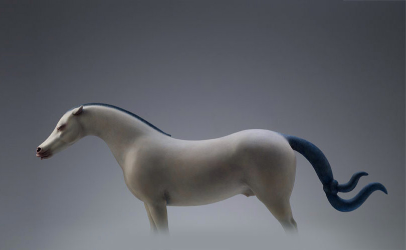
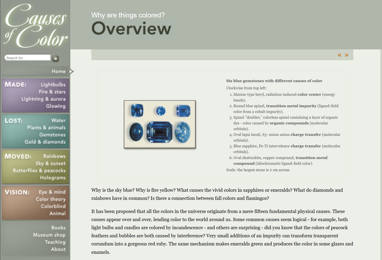
What causes color
Read more: What causes colorwww.webexhibits.org/causesofcolor/5.html
Water itself has an intrinsic blue color that is a result of its molecular structure and its behavior.
-
Anders Langlands – Render Color Spaces
Read more: Anders Langlands – Render Color Spaceshttps://www.colour-science.org/anders-langlands/
This page compares images rendered in Arnold using spectral rendering and different sets of colourspace primaries: Rec.709, Rec.2020, ACES and DCI-P3. The SPD data for the GretagMacbeth Color Checker are the measurements of Noburu Ohta, taken from Mansencal, Mauderer and Parsons (2014) colour-science.org.

-
If a blind person gained sight, could they recognize objects previously touched?
Read more: If a blind person gained sight, could they recognize objects previously touched?Blind people who regain their sight may find themselves in a world they don’t immediately comprehend. “It would be more like a sighted person trying to rely on tactile information,” Moore says.
Learning to see is a developmental process, just like learning language, Prof Cathleen Moore continues. “As far as vision goes, a three-and-a-half year old child is already a well-calibrated system.”
-
sRGB vs REC709 – An introduction and FFmpeg implementations
Read more: sRGB vs REC709 – An introduction and FFmpeg implementations
1. Basic Comparison
- What they are
- sRGB: A standard “web”/computer-display RGB color space defined by IEC 61966-2-1. It’s used for most monitors, cameras, printers, and the vast majority of images on the Internet.
- Rec. 709: An HD-video color space defined by ITU-R BT.709. It’s the go-to standard for HDTV broadcasts, Blu-ray discs, and professional video pipelines.
- Why they exist
- sRGB: Ensures consistent colors across different consumer devices (PCs, phones, webcams).
- Rec. 709: Ensures consistent colors across video production and playback chains (cameras → editing → broadcast → TV).
- What you’ll see
- On your desktop or phone, images tagged sRGB will look “right” without extra tweaking.
- On an HDTV or video-editing timeline, footage tagged Rec. 709 will display accurate contrast and hue on broadcast-grade monitors.
2. Digging Deeper
Feature sRGB Rec. 709 White point D65 (6504 K), same for both D65 (6504 K) Primaries (x,y) R: (0.640, 0.330) G: (0.300, 0.600) B: (0.150, 0.060) R: (0.640, 0.330) G: (0.300, 0.600) B: (0.150, 0.060) Gamut size Identical triangle on CIE 1931 chart Identical to sRGB Gamma / transfer Piecewise curve: approximate 2.2 with linear toe Pure power-law γ≈2.4 (often approximated as 2.2 in practice) Matrix coefficients N/A (pure RGB usage) Y = 0.2126 R + 0.7152 G + 0.0722 B (Rec. 709 matrix) Typical bit-depth 8-bit/channel (with 16-bit variants) 8-bit/channel (10-bit for professional video) Usage metadata Tagged as “sRGB” in image files (PNG, JPEG, etc.) Tagged as “bt709” in video containers (MP4, MOV) Color range Full-range RGB (0–255) Studio-range Y′CbCr (Y′ [16–235], Cb/Cr [16–240])
Why the Small Differences Matter
(more…) - What they are
-
A Brief History of Color in Art
Read more: A Brief History of Color in Artwww.artsy.net/article/the-art-genome-project-a-brief-history-of-color-in-art
Of all the pigments that have been banned over the centuries, the color most missed by painters is likely Lead White.
This hue could capture and reflect a gleam of light like no other, though its production was anything but glamorous. The 17th-century Dutch method for manufacturing the pigment involved layering cow and horse manure over lead and vinegar. After three months in a sealed room, these materials would combine to create flakes of pure white. While scientists in the late 19th century identified lead as poisonous, it wasn’t until 1978 that the United States banned the production of lead white paint.

More reading:
www.canva.com/learn/color-meanings/https://www.infogrades.com/history-events-infographics/bizarre-history-of-colors/

-
Scene Referred vs Display Referred color workflows
Read more: Scene Referred vs Display Referred color workflowsDisplay Referred it is tied to the target hardware, as such it bakes color requirements into every type of media output request.
Scene Referred uses a common unified wide gamut and targeting audience through CDL and DI libraries instead.
So that color information stays untouched and only “transformed” as/when needed.


Sources:
– Victor Perez – Color Management Fundamentals & ACES Workflows in Nuke
– https://z-fx.nl/ColorspACES.pdf
– Wicus


LIGHTING
-
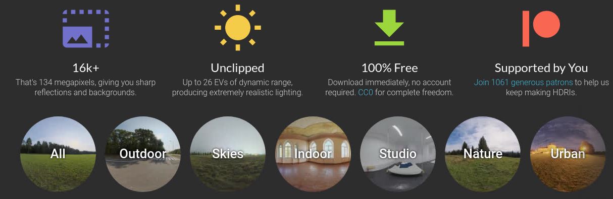
Free HDRI libraries
Read more: Free HDRI librariesnoahwitchell.com
http://www.noahwitchell.com/freebieslocationtextures.com
https://locationtextures.com/panoramas/maxroz.com
https://www.maxroz.com/hdri/listHDRI Haven
https://hdrihaven.com/Poly Haven
https://polyhaven.com/hdrisDomeble
https://www.domeble.com/IHDRI
https://www.ihdri.com/HDRMaps
https://hdrmaps.com/NoEmotionHdrs.net
http://noemotionhdrs.net/hdrday.htmlOpenFootage.net
https://www.openfootage.net/hdri-panorama/HDRI-hub
https://www.hdri-hub.com/hdrishop/hdri.zwischendrin
https://www.zwischendrin.com/en/browse/hdriLonger list here:
https://cgtricks.com/list-sites-free-hdri/
-
Photography basics: Lumens vs Candelas (candle) vs Lux vs FootCandle vs Watts vs Irradiance vs Illuminance
Read more: Photography basics: Lumens vs Candelas (candle) vs Lux vs FootCandle vs Watts vs Irradiance vs Illuminancehttps://www.translatorscafe.com/unit-converter/en-US/illumination/1-11/

The power output of a light source is measured using the unit of watts W. This is a direct measure to calculate how much power the light is going to drain from your socket and it is not relatable to the light brightness itself.
The amount of energy emitted from it per second. That energy comes out in a form of photons which we can crudely represent with rays of light coming out of the source. The higher the power the more rays emitted from the source in a unit of time.
Not all energy emitted is visible to the human eye, so we often rely on photometric measurements, which takes in account the sensitivity of human eye to different wavelenghts


Details in the post
(more…) -
Willem Zwarthoed – Aces gamut in VFX production pdf
Read more: Willem Zwarthoed – Aces gamut in VFX production pdfhttps://www.provideocoalition.com/color-management-part-12-introducing-aces/
Local copy:
https://www.slideshare.net/hpduiker/acescg-a-common-color-encoding-for-visual-effects-applications
-
Romain Chauliac – LightIt a lighting script for Maya and Arnold
Read more: Romain Chauliac – LightIt a lighting script for Maya and ArnoldLightIt is a script for Maya and Arnold that will help you and improve your lighting workflow.
Thanks to preset studio lighting components (lights, backdrop…), high quality studio scenes and HDRI library manager.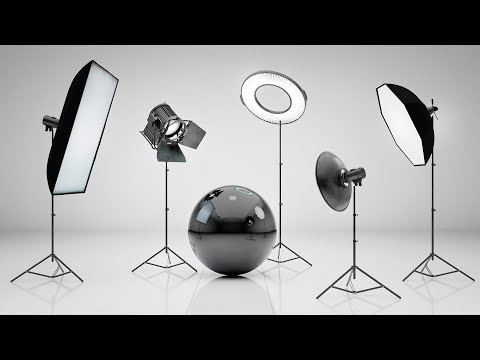
https://www.artstation.com/artwork/393emJ
-
Open Source Nvidia Omniverse
Read more: Open Source Nvidia Omniverseblogs.nvidia.com/blog/2019/03/18/omniverse-collaboration-platform/
developer.nvidia.com/nvidia-omniverse
An open, Interactive 3D Design Collaboration Platform for Multi-Tool Workflows to simplify studio workflows for real-time graphics.
It supports Pixar’s Universal Scene Description technology for exchanging information about modeling, shading, animation, lighting, visual effects and rendering across multiple applications.
It also supports NVIDIA’s Material Definition Language, which allows artists to exchange information about surface materials across multiple tools.
With Omniverse, artists can see live updates made by other artists working in different applications. They can also see changes reflected in multiple tools at the same time.
For example an artist using Maya with a portal to Omniverse can collaborate with another artist using UE4 and both will see live updates of each others’ changes in their application.
-
domeble – Hi-Resolution CGI Backplates and 360° HDRI
Read more: domeble – Hi-Resolution CGI Backplates and 360° HDRIWhen collecting hdri make sure the data supports basic metadata, such as:
- Iso
- Aperture
- Exposure time or shutter time
- Color temperature
- Color space Exposure value (what the sensor receives of the sun intensity in lux)
- 7+ brackets (with 5 or 6 being the perceived balanced exposure)
In image processing, computer graphics, and photography, high dynamic range imaging (HDRI or just HDR) is a set of techniques that allow a greater dynamic range of luminances (a Photometry measure of the luminous intensity per unit area of light travelling in a given direction. It describes the amount of light that passes through or is emitted from a particular area, and falls within a given solid angle) between the lightest and darkest areas of an image than standard digital imaging techniques or photographic methods. This wider dynamic range allows HDR images to represent more accurately the wide range of intensity levels found in real scenes ranging from direct sunlight to faint starlight and to the deepest shadows.
The two main sources of HDR imagery are computer renderings and merging of multiple photographs, which in turn are known as low dynamic range (LDR) or standard dynamic range (SDR) images. Tone Mapping (Look-up) techniques, which reduce overall contrast to facilitate display of HDR images on devices with lower dynamic range, can be applied to produce images with preserved or exaggerated local contrast for artistic effect. Photography
In photography, dynamic range is measured in Exposure Values (in photography, exposure value denotes all combinations of camera shutter speed and relative aperture that give the same exposure. The concept was developed in Germany in the 1950s) differences or stops, between the brightest and darkest parts of the image that show detail. An increase of one EV or one stop is a doubling of the amount of light.
The human response to brightness is well approximated by a Steven’s power law, which over a reasonable range is close to logarithmic, as described by the Weber�Fechner law, which is one reason that logarithmic measures of light intensity are often used as well.
HDR is short for High Dynamic Range. It’s a term used to describe an image which contains a greater exposure range than the “black” to “white” that 8 or 16-bit integer formats (JPEG, TIFF, PNG) can describe. Whereas these Low Dynamic Range images (LDR) can hold perhaps 8 to 10 f-stops of image information, HDR images can describe beyond 30 stops and stored in 32 bit images.


COLLECTIONS
| Featured AI
| Design And Composition
| Explore posts
POPULAR SEARCHES
unreal | pipeline | virtual production | free | learn | photoshop | 360 | macro | google | nvidia | resolution | open source | hdri | real-time | photography basics | nuke
FEATURED POSTS
-
Zibra.AI – Real-Time Volumetric Effects in Virtual Production. Now free for Indies!
-
copypastecharacter.com – alphabets, special characters, alt codes and symbols library
-
Blender VideoDepthAI – Turn any video into 3D Animated Scenes
-
Godot Cheat Sheets
-
The Public Domain Is Working Again — No Thanks To Disney
-
Matt Gray – How to generate a profitable business
-
WhatDreamsCost Spline-Path-Control – Create motion controls for ComfyUI
-
UV maps
Social Links
DISCLAIMER – Links and images on this website may be protected by the respective owners’ copyright. All data submitted by users through this site shall be treated as freely available to share.
