ACES 2.0 is the second major release of the components that make up the ACES system. The most significant change is a new suite of rendering transforms whose design was informed by collected feedback and requests from users of ACES 1. The changes aim to improve the appearance of perceived artifacts and to complete previously unfinished components of the system, resulting in a more complete, robust, and consistent product.
Highlights of the key changes in ACES 2.0 are as follows:
New output transforms, including:
A less aggressive tone scale
More intuitive controls to create custom outputs to non-standard displays
Robust gamut mapping to improve perceptual uniformity
Improved performance of the inverse transforms
Enhanced AMF specification
An updated specification for ACES Transform IDs
OpenEXR compression recommendations
Enhanced tools for generating Input Transforms and recommended procedures for characterizing prosumer cameras
Look Transform Library
Expanded documentation
Rendering Transform
The most substantial change in ACES 2.0 is a complete redesign of the rendering transform.
ACES 2.0 was built as a unified system, rather than through piecemeal additions. Different deliverable outputs “match” better and making outputs to display setups other than the provided presets is intended to be user-driven. The rendering transforms are less likely to produce undesirable artifacts “out of the box”, which means less time can be spent fixing problematic images and more time making pictures look the way you want.
Key design goals
Improve consistency of tone scale and provide an easy to use parameter to allow for outputs between preset dynamic ranges
Minimize hue skews across exposure range in a region of same hue
Unify for structural consistency across transform type
Easy to use parameters to create outputs other than the presets
Robust gamut mapping to improve harsh clipping artifacts
Fill extents of output code value cube (where appropriate and expected)
Invertible – not necessarily reversible, but Output > ACES > Output round-trip should be possible
Accomplish all of the above while maintaining an acceptable “out-of-the box” rendering
In color technology, color depth also known as bit depth, is either the number of bits used to indicate the color of a single pixel, OR the number of bits used for each color component of a single pixel.
When referring to a pixel, the concept can be defined as bits per pixel (bpp).
When referring to a color component, the concept can be defined as bits per component, bits per channel, bits per color (all three abbreviated bpc), and also bits per pixel component, bits per color channel or bits per sample (bps). Modern standards tend to use bits per component, but historical lower-depth systems used bits per pixel more often.
Color depth is only one aspect of color representation, expressing the precision with which the amount of each primary can be expressed; the other aspect is how broad a range of colors can be expressed (the gamut). The definition of both color precision and gamut is accomplished with a color encoding specification which assigns a digital code value to a location in a color space.
In HD we often refer to the range of available colors as a color gamut. Such a color gamut is typically plotted on a two-dimensional diagram, called a CIE chart, as shown in at the top of this blog. Each color is characterized by its x/y coordinates.
Good enough for government work, perhaps. But for HDR, with its higher luminance levels and wider color, the gamut becomes three-dimensional.
For HDR the color gamut therefore becomes a characteristic we now call the color volume. It isn’t easy to show color volume on a two-dimensional medium like the printed page or a computer screen, but one method is shown below. As the luminance becomes higher, the picture eventually turns to white. As it becomes darker, it fades to black. The traditional color gamut shown on the CIE chart is simply a slice through this color volume at a selected luminance level, such as 50%.
Three different color volumes—we still refer to them as color gamuts though their third dimension is important—are currently the most significant. The first is BT.709 (sometimes referred to as Rec.709), the color gamut used for pre-UHD/HDR formats, including standard HD.
The largest is known as BT.2020; it encompasses (roughly) the range of colors visible to the human eye (though ET might find it insufficient!).
Between these two is the color gamut used in digital cinema, known as DCI-P3.
Of all the pigments that have been banned over the centuries, the color most missed by painters is likely Lead White.
This hue could capture and reflect a gleam of light like no other, though its production was anything but glamorous. The 17th-century Dutch method for manufacturing the pigment involved layering cow and horse manure over lead and vinegar. After three months in a sealed room, these materials would combine to create flakes of pure white. While scientists in the late 19th century identified lead as poisonous, it wasn’t until 1978 that the United States banned the production of lead white paint.
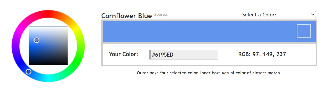
Björn Ottosson proposed OKlch in 2020 to create a color space that can closely mimic how color is perceived by the human eye, predicting perceived lightness, chroma, and hue.
The OK in OKLCH stands for Optimal Color.
L: Lightness (the perceived brightness of the color)
C: Chroma (the intensity or saturation of the color)
H: Hue (the actual color, such as red, blue, green, etc.)
One problem with sRGB is that in a gradient between blue and white, it becomes a bit purple in the middle of the transition. That’s because sRGB really isn’t created to mimic how the eye sees colors; rather, it is based on how CRT monitors work. That means it works with certain frequencies of red, green, and blue, and also the non-linear coding called gamma. It’s a miracle it works as well as it does, but it’s not connected to color perception. When using those tools, you sometimes get surprising results, like purple in the gradient.
There were also attempts to create simple models matching human perception based on XYZ, but as it turned out, it’s not possible to model all color vision that way. Perception of color is incredibly complex and depends, among other things, on whether it is dark or light in the room and the background color it is against. When you look at a photograph, it also depends on what you think the color of the light source is. The dress is a typical example of color vision being very context-dependent. It is almost impossible to model this perfectly.
I based Oklab on two other color spaces, CIECAM16 and IPT. I used the lightness and saturation prediction from CIECAM16, which is a color appearance model, as a target. I actually wanted to use the datasets used to create CIECAM16, but I couldn’t find them.
IPT was designed to have better hue uniformity. In experiments, they asked people to match light and dark colors, saturated and unsaturated colors, which resulted in a dataset for which colors, subjectively, have the same hue. IPT has a few other issues but is the basis for hue in Oklab.
In the Munsell color system, colors are described with three parameters, designed to match the perceived appearance of colors: Hue, Chroma and Value. The parameters are designed to be independent and each have a uniform scale. This results in a color solid with an irregular shape. The parameters are designed to be independent and each have a uniform scale. This results in a color solid with an irregular shape. Modern color spaces and models, such as CIELAB, Cam16 and Björn Ottosson own Oklab, are very similar in their construction.
By far the most used color spaces today for color picking are HSL and HSV, two representations introduced in the classic 1978 paper “Color Spaces for Computer Graphics”. HSL and HSV designed to roughly correlate with perceptual color properties while being very simple and cheap to compute.
Today HSL and HSV are most commonly used together with the sRGB color space.
One of the main advantages of HSL and HSV over the different Lab color spaces is that they map the sRGB gamut to a cylinder. This makes them easy to use since all parameters can be changed independently, without the risk of creating colors outside of the target gamut.
The main drawback on the other hand is that their properties don’t match human perception particularly well.
Reconciling these conflicting goals perfectly isn’t possible, but given that HSV and HSL don’t use anything derived from experiments relating to human perception, creating something that makes a better tradeoff does not seem unreasonable.
With this new lightness estimate, we are ready to look into the construction of Okhsv and Okhsl.
A light wave that is vibrating in more than one plane is referred to as unpolarized light. …
Polarized light waves are light waves in which the vibrations occur in a single plane. The process of transforming unpolarized light into polarized light is known as polarization.
The most common use of polarized technology is to reduce lighting complexity on the subject. Details such as glare and hard edges are not removed, but greatly reduced.
By stimulating specific cells in the retina, the participants claim to have witnessed a blue-green colour that scientists have called “olo”, but some experts have said the existence of a new colour is “open to argument”.
The findings, published in the journal Science Advances on Friday, have been described by the study’s co-author, Prof Ren Ng from the University of California, as “remarkable”.
(A) System inputs. (i) Retina map of 103 cone cells preclassified by spectral type (7). (ii) Target visual percept (here, a video of a child, see movie S1 at 1:04). (iii) Infrared cellular-scale imaging of the retina with 60-frames-per-second rolling shutter. Fixational eye movement is visible over the three frames shown.
(B) System outputs. (iv) Real-time per-cone target activation levels to reproduce the target percept, computed by: extracting eye motion from the input video relative to the retina map; identifying the spectral type of every cone in the field of view; computing the per-cone activation the target percept would have produced. (v) Intensities of visible-wavelength 488-nm laser microdoses at each cone required to achieve its target activation level.
(C) Infrared imaging and visible-wavelength stimulation are physically accomplished in a raster scan across the retinal region using AOSLO. By modulating the visible-wavelength beam’s intensity, the laser microdoses shown in (v) are delivered. Drawing adapted with permission [Harmening and Sincich (54)].
(D) Examples of target percepts with corresponding cone activations and laser microdoses, ranging from colored squares to complex imagery. Teal-striped regions represent the color “olo” of stimulating only M cones.
Physically-based shading means leaving behind phenomenological models, like the Phong shading model, which are simply built to “look good” subjectively without being based on physics in any real way, and moving to lighting and shading models that are derived from the laws of physics and/or from actual measurements of the real world, and rigorously obey physical constraints such as energy conservation.
For example, in many older rendering systems, shading models included separate controls for specular highlights from point lights and reflection of the environment via a cubemap. You could create a shader with the specular and the reflection set to wildly different values, even though those are both instances of the same physical process. In addition, you could set the specular to any arbitrary brightness, even if it would cause the surface to reflect more energy than it actually received.
In a physically-based system, both the point light specular and the environment reflection would be controlled by the same parameter, and the system would be set up to automatically adjust the brightness of both the specular and diffuse components to maintain overall energy conservation. Moreover you would want to set the specular brightness to a realistic value for the material you’re trying to simulate, based on measurements.
Physically-based lighting or shading includes physically-based BRDFs, which are usually based on microfacet theory, and physically correct light transport, which is based on the rendering equation (although heavily approximated in the case of real-time games).
It also includes the necessary changes in the art process to make use of these features. Switching to a physically-based system can cause some upsets for artists. First of all it requires full HDR lighting with a realistic level of brightness for light sources, the sky, etc. and this can take some getting used to for the lighting artists. It also requires texture/material artists to do some things differently (particularly for specular), and they can be frustrated by the apparent loss of control (e.g. locking together the specular highlight and environment reflection as mentioned above; artists will complain about this). They will need some time and guidance to adapt to the physically-based system.
On the plus side, once artists have adapted and gained trust in the physically-based system, they usually end up liking it better, because there are fewer parameters overall (less work for them to tweak). Also, materials created in one lighting environment generally look fine in other lighting environments too. This is unlike more ad-hoc models, where a set of material parameters might look good during daytime, but it comes out ridiculously glowy at night, or something like that.
Here are some resources to look at for physically-based lighting in games:
SIGGRAPH 2013 Physically Based Shading Course, particularly the background talk by Naty Hoffman at the beginning. You can also check out the previous incarnations of this course for more resources.
And of course, I would be remiss if I didn’t mention Physically-Based Rendering by Pharr and Humphreys, an amazing reference on this whole subject and well worth your time, although it focuses on offline rather than real-time rendering.
“a simple yet effective technique to estimate lighting in a single input image. Current techniques rely heavily on HDR panorama datasets to train neural networks to regress an input with limited field-of-view to a full environment map. However, these approaches often struggle with real-world, uncontrolled settings due to the limited diversity and size of their datasets. To address this problem, we leverage diffusion models trained on billions of standard images to render a chrome ball into the input image. Despite its simplicity, this task remains challenging: the diffusion models often insert incorrect or inconsistent objects and cannot readily generate images in HDR format. Our research uncovers a surprising relationship between the appearance of chrome balls and the initial diffusion noise map, which we utilize to consistently generate high-quality chrome balls. We further fine-tune an LDR difusion model (Stable Diffusion XL) with LoRA, enabling it to perform exposure bracketing for HDR light estimation. Our method produces convincing light estimates across diverse settings and demonstrates superior generalization to in-the-wild scenarios.”
DISCLAIMER – Links and images on this website may be protected by the respective owners’ copyright. All data submitted by users through this site shall be treated as freely available to share.


