


COMPOSITION
DESIGN
-
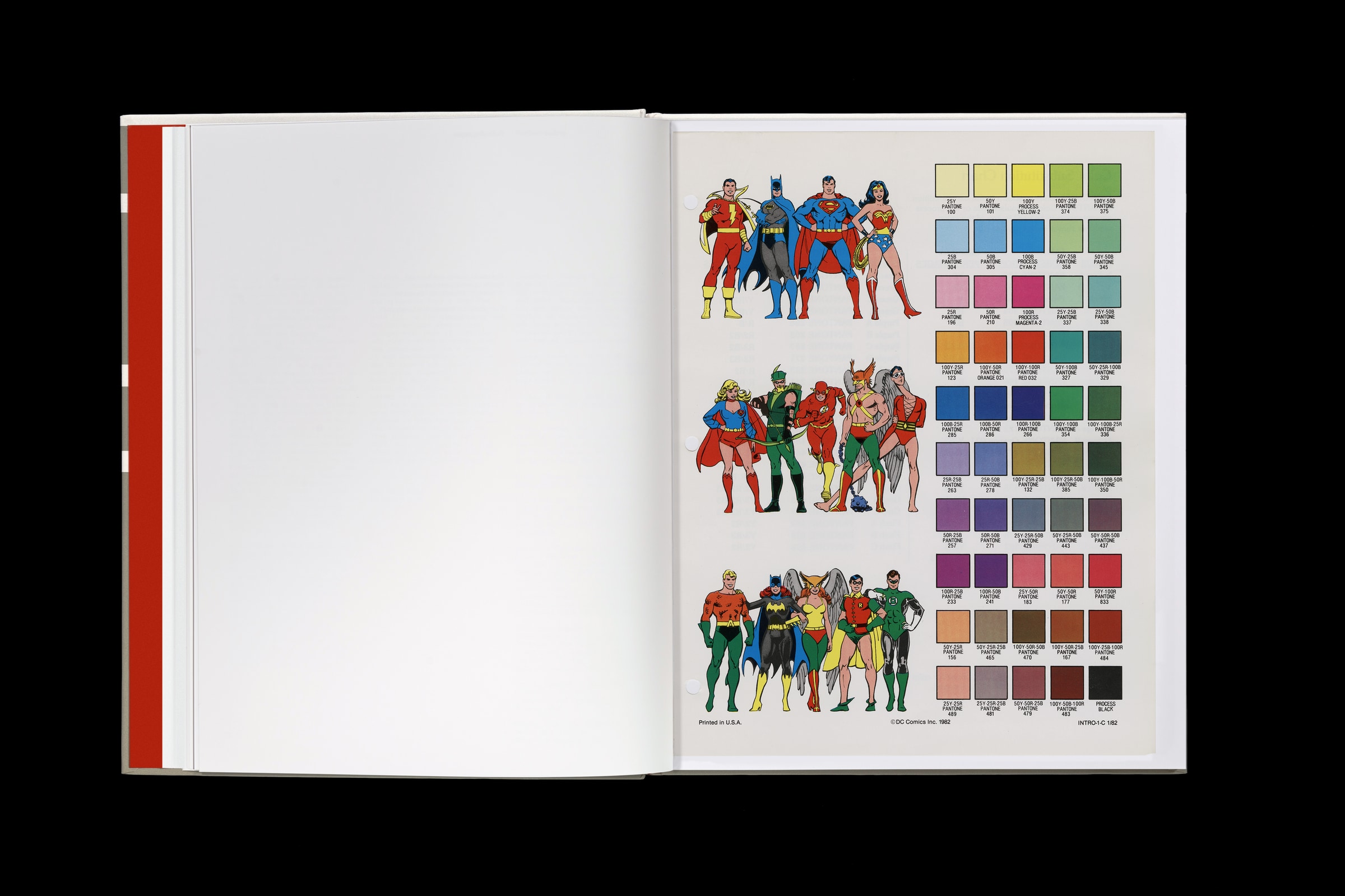
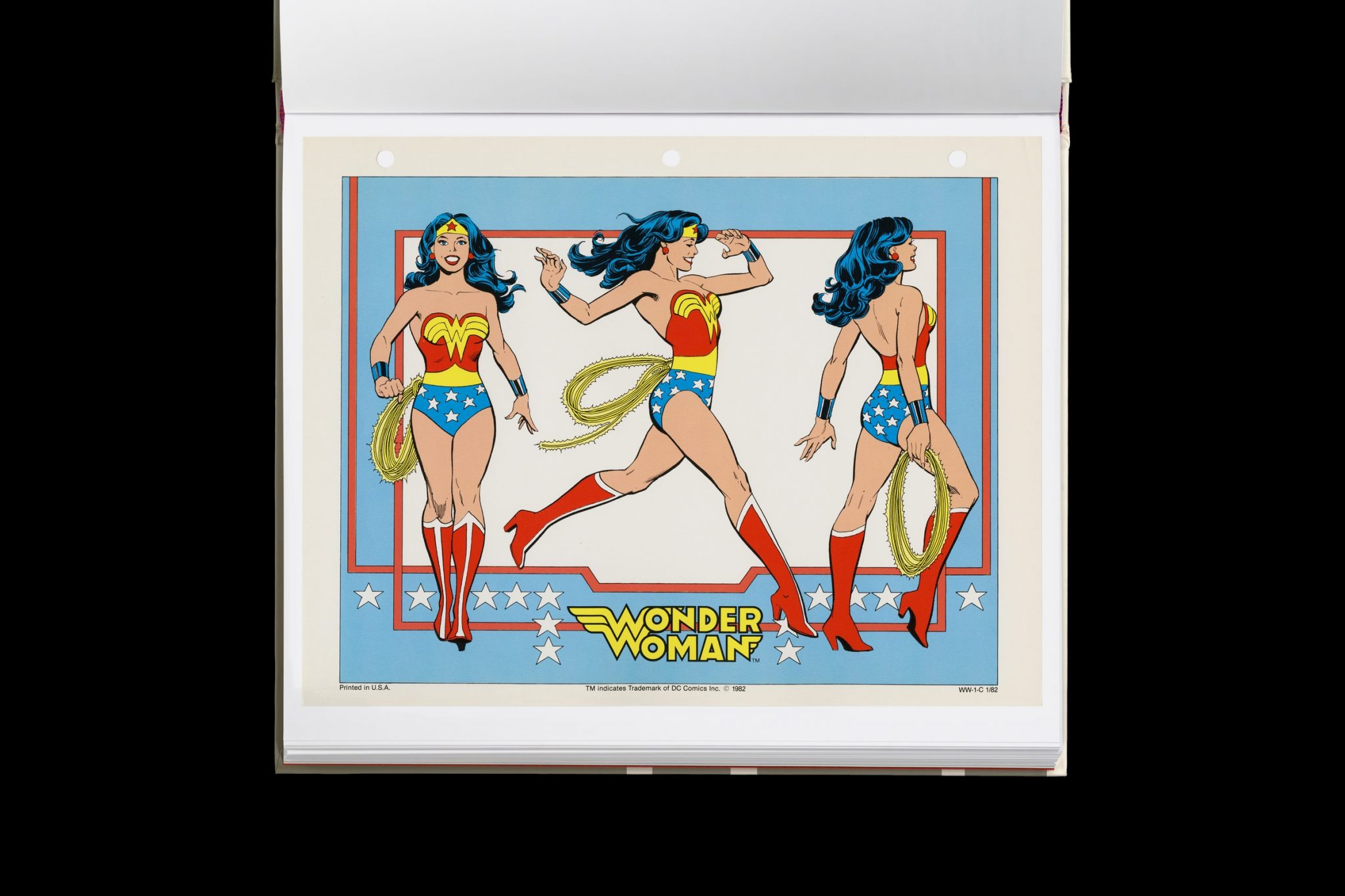
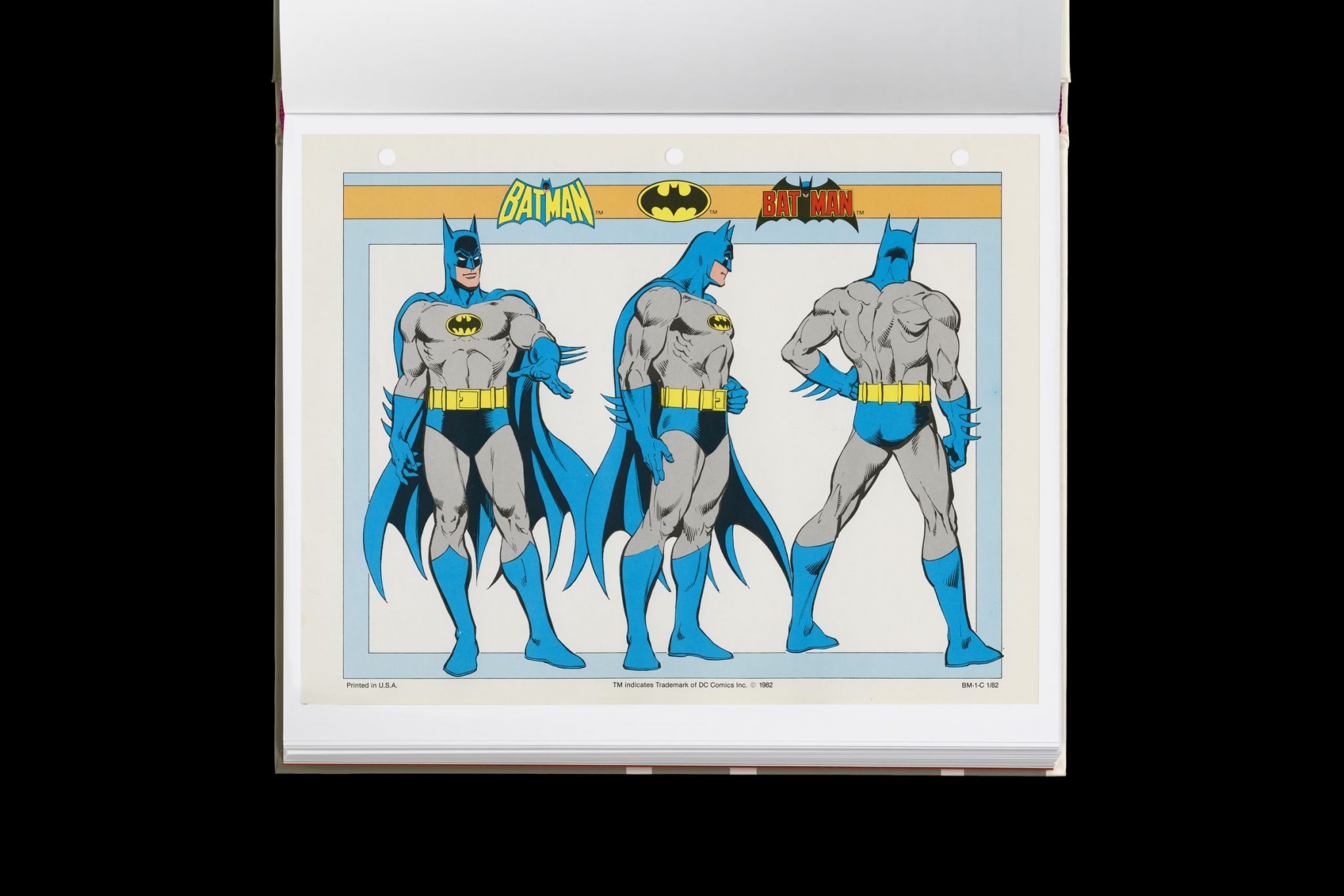
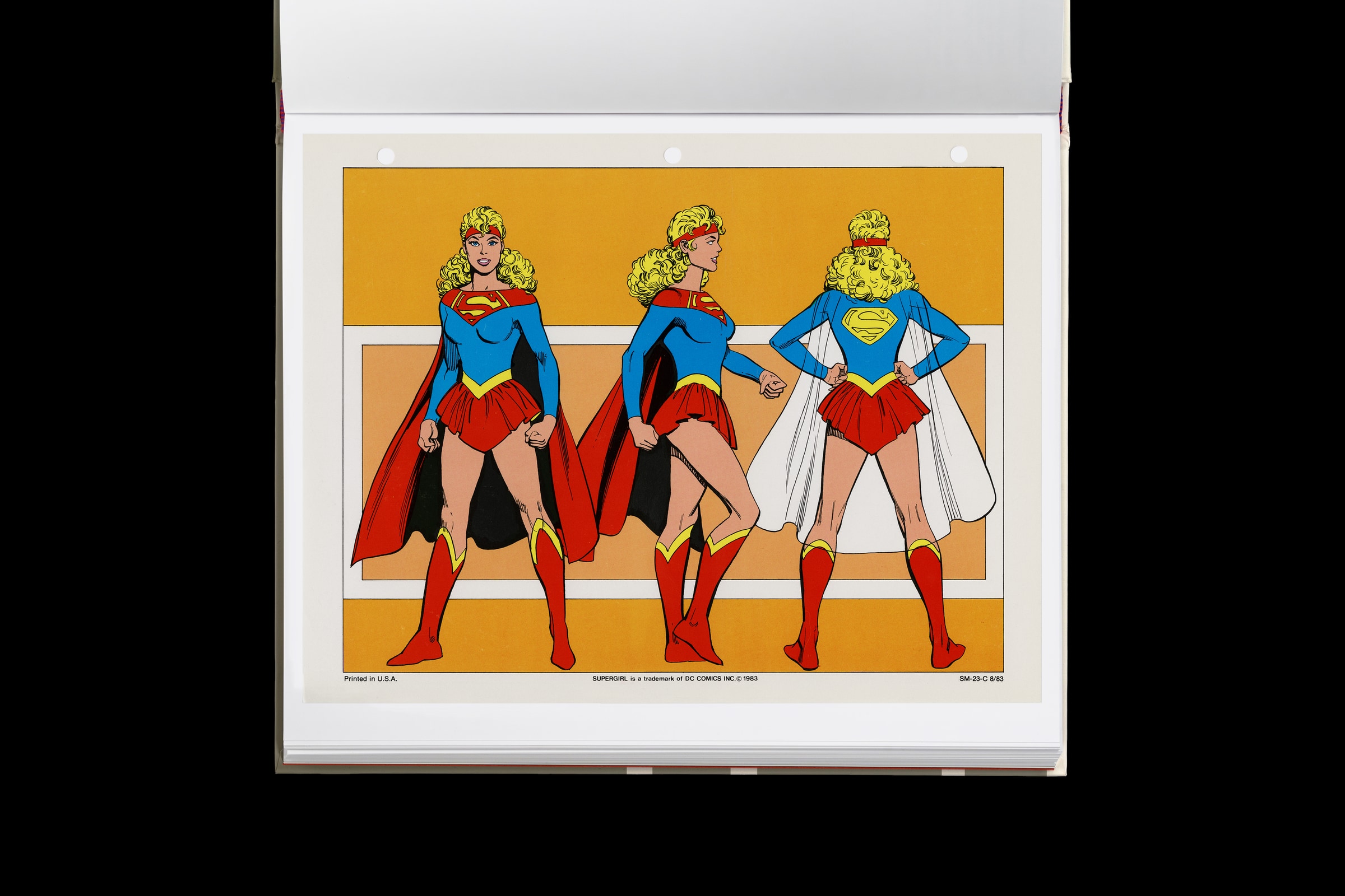
This legendary DC Comics style guide was nearly lost for years – now you can buy it
Read more: This legendary DC Comics style guide was nearly lost for years – now you can buy ithttps://www.fastcompany.com/91133306/dc-comics-style-guide-was-lost-for-years-now-you-can-buy-it
Reproduced from a rare original copy, the book features over 165 highly-detailed scans of the legendary art by José Luis García-López, with an introduction by Paul Levitz, former president of DC Comics.
https://standardsmanual.com/products/1982-dc-comics-style-guide
-
Principles of Interior Design – Balance
Read more: Principles of Interior Design – Balancehttps://www.yankodesign.com/2024/09/18/principles-of-interior-design-balance
The three types of balance include:
- Symmetrical Balance
- Asymmetrical Balance
- Radial Balance
-
Pantheon of the War – The colossal war painting
Read more: Pantheon of the War – The colossal war paintingFour years in the making with the help of 150 artists, in commemoration of WW1.
edition.cnn.com/style/article/pantheon-de-la-guerre-wwi-painting/index.html
A panoramic canvas measuring 402 feet (122 meters) around and 45 feet (13.7 meters) high. It contained over 5,000 life-size portraits of war heroes, royalty and government officials from the Allies of World War I.
Partial section upload:


COLOR
-
Victor Perez – The Color Management Handbook for Visual Effects Artists
Read more: Victor Perez – The Color Management Handbook for Visual Effects ArtistsDigital Color Principles, Color Management Fundamentals & ACES Workflows

-
What light is best to illuminate gems for resale
Read more: What light is best to illuminate gems for resalewww.palagems.com/gem-lighting2
Artificial light sources, not unlike the diverse phases of natural light, vary considerably in their properties. As a result, some lamps render an object’s color better than others do.
The most important criterion for assessing the color-rendering ability of any lamp is its spectral power distribution curve.
Natural daylight varies too much in strength and spectral composition to be taken seriously as a lighting standard for grading and dealing colored stones. For anything to be a standard, it must be constant in its properties, which natural light is not.
For dealers in particular to make the transition from natural light to an artificial light source, that source must offer:
1- A degree of illuminance at least as strong as the common phases of natural daylight.
2- Spectral properties identical or comparable to a phase of natural daylight.A source combining these two things makes gems appear much the same as when viewed under a given phase of natural light. From the viewpoint of many dealers, this corresponds to a naturalappearance.
The 6000° Kelvin xenon short-arc lamp appears closest to meeting the criteria for a standard light source. Besides the strong illuminance this lamp affords, its spectrum is very similar to CIE standard illuminants of similar color temperature.


-
PBR Color Reference List for Materials – by Grzegorz Baran
Read more: PBR Color Reference List for Materials – by Grzegorz Baran
“The list should be helpful for every material artist who work on PBR materials as it contains over 200 color values measured with PCE-RGB2 1002 Color Spectrometer device and presented in linear and sRGB (2.2) gamma space.
All color values, HUE and Saturation in this list come from measurements taken with PCE-RGB2 1002 Color Spectrometer device and are presented in linear and sRGB (2.2) gamma space (more info at the end of this video) I calculated Relative Luminance and Luminance values based on captured color using my own equation which takes color based luminance perception into consideration. Bare in mind that there is no ‘one’ color per substance as nothing in nature is even 100% uniform and any value in +/-10% range from these should be considered as correct one. Therefore this list should be always considered as a color reference for material’s albedos, not ulitimate and absolute truth.“
-
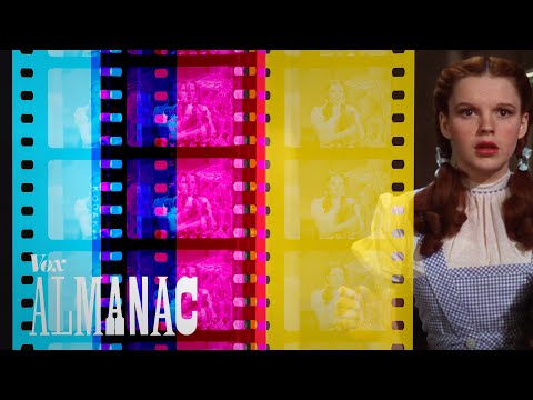
The Color of Infinite Temperature
Read more: The Color of Infinite TemperatureThis is the color of something infinitely hot.

Of course you’d instantly be fried by gamma rays of arbitrarily high frequency, but this would be its spectrum in the visible range.
johncarlosbaez.wordpress.com/2022/01/16/the-color-of-infinite-temperature/
This is also the color of a typical neutron star. They’re so hot they look the same.
It’s also the color of the early Universe!This was worked out by David Madore.

The color he got is sRGB(148,177,255).
www.htmlcsscolor.com/hex/94B1FFAnd according to the experts who sip latte all day and make up names for colors, this color is called ‘Perano’.


LIGHTING
-
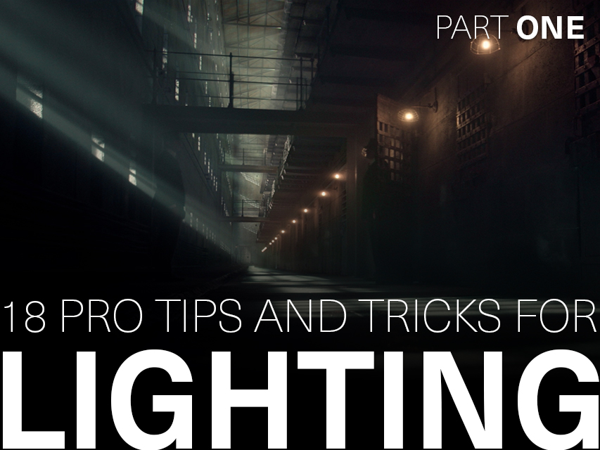
Outpost VFX lighting tips
Read more: Outpost VFX lighting tipswww.outpost-vfx.com/en/news/18-pro-tips-and-tricks-for-lighting
Get as much information regarding your plate lighting as possible
- Always use a reference
- Replicate what is happening in real life
- Invest into a solid HDRI
- Start Simple
- Observe real world lighting, photography and cinematography
- Don’t neglect the theory
- Learn the difference between realism and photo-realism.
- Keep your scenes organised
-
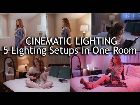
7 Easy Portrait Lighting Setups
Read more: 7 Easy Portrait Lighting Setups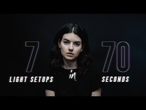
Butterfly
Loop
Rembrandt
Split
Rim
Broad
Short
-
Composition – cinematography Cheat Sheet
Read more: Composition – cinematography Cheat Sheet
Where is our eye attracted first? Why?
Size. Focus. Lighting. Color.
Size. Mr. White (Harvey Keitel) on the right.
Focus. He’s one of the two objects in focus.
Lighting. Mr. White is large and in focus and Mr. Pink (Steve Buscemi) is highlighted by
a shaft of light.
Color. Both are black and white but the read on Mr. White’s shirt now really stands out.
(more…)
What type of lighting? -
Rendering – BRDF – Bidirectional reflectance distribution function
Read more: Rendering – BRDF – Bidirectional reflectance distribution functionhttp://en.wikipedia.org/wiki/Bidirectional_reflectance_distribution_function
The bidirectional reflectance distribution function is a four-dimensional function that defines how light is reflected at an opaque surface
http://www.cs.ucla.edu/~zhu/tutorial/An_Introduction_to_BRDF-Based_Lighting.pdf
In general, when light interacts with matter, a complicated light-matter dynamic occurs. This interaction depends on the physical characteristics of the light as well as the physical composition and characteristics of the matter.
That is, some of the incident light is reflected, some of the light is transmitted, and another portion of the light is absorbed by the medium itself.
A BRDF describes how much light is reflected when light makes contact with a certain material. Similarly, a BTDF (Bi-directional Transmission Distribution Function) describes how much light is transmitted when light makes contact with a certain material
http://www.cs.princeton.edu/~smr/cs348c-97/surveypaper.html
It is difficult to establish exactly how far one should go in elaborating the surface model. A truly complete representation of the reflective behavior of a surface might take into account such phenomena as polarization, scattering, fluorescence, and phosphorescence, all of which might vary with position on the surface. Therefore, the variables in this complete function would be:
incoming and outgoing angle incoming and outgoing wavelength incoming and outgoing polarization (both linear and circular) incoming and outgoing position (which might differ due to subsurface scattering) time delay between the incoming and outgoing light ray

![[gamma correction test]](http://www.madore.org/~david/misc/color/gammatest.png "sRGB gamma correction test")


COLLECTIONS
| Featured AI
| Design And Composition
| Explore posts
POPULAR SEARCHES
unreal | pipeline | virtual production | free | learn | photoshop | 360 | macro | google | nvidia | resolution | open source | hdri | real-time | photography basics | nuke
FEATURED POSTS
Social Links
DISCLAIMER – Links and images on this website may be protected by the respective owners’ copyright. All data submitted by users through this site shall be treated as freely available to share.
