


COMPOSITION
DESIGN
-
Myriam Catrin – amazing design
Read more: Myriam Catrin – amazing designhttps://www.artstation.com/myriamcatrin
Creator of the comic book ” Passages. Book I” released with @therealarttitude
https://arttitudebootleg.bigcartel.com/product/passages-myriam-catrin
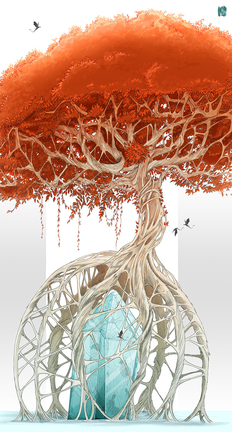
instagram/ FB page: @myriamcatrin / @MyriamCatrinComics
-
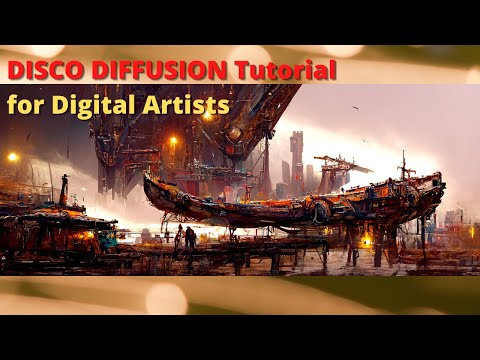
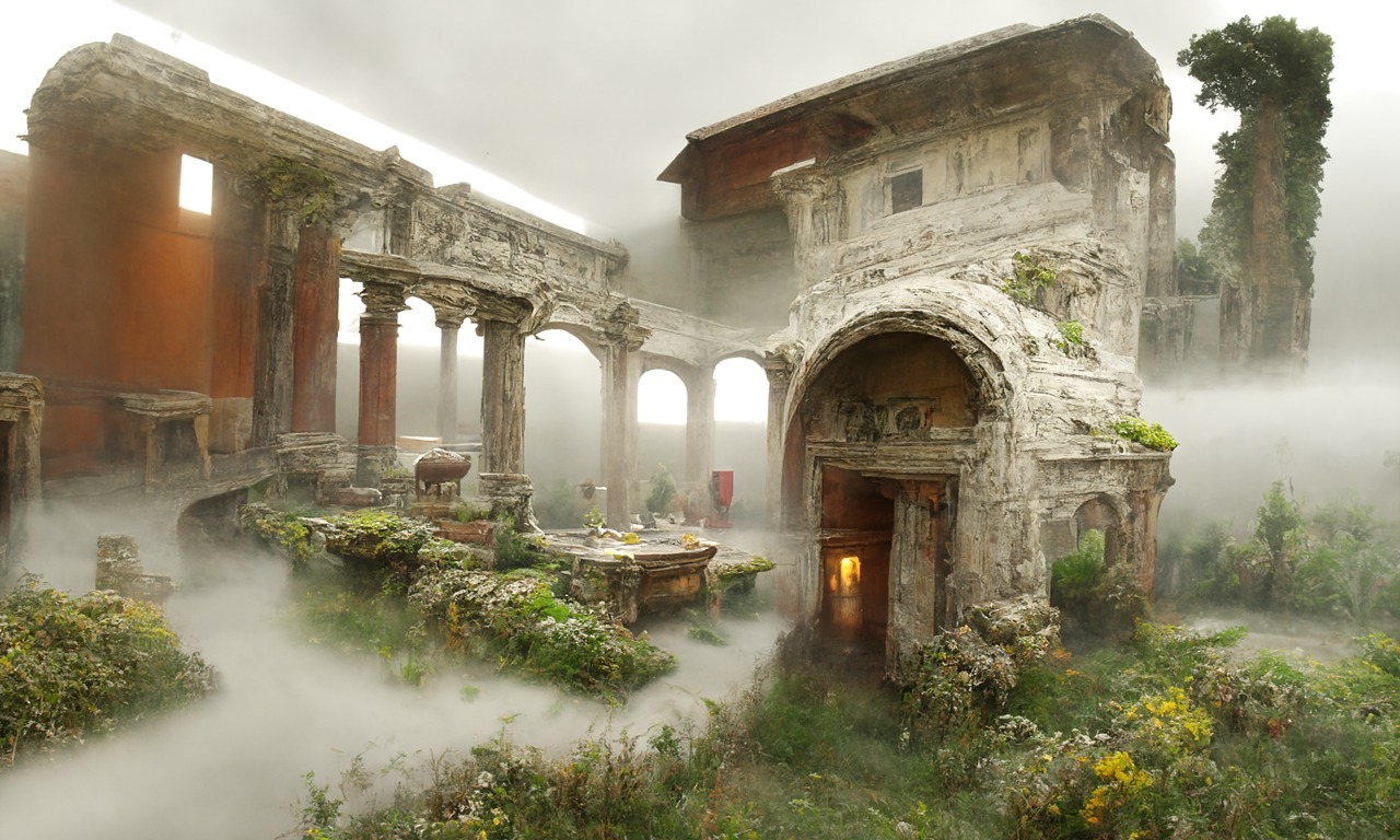
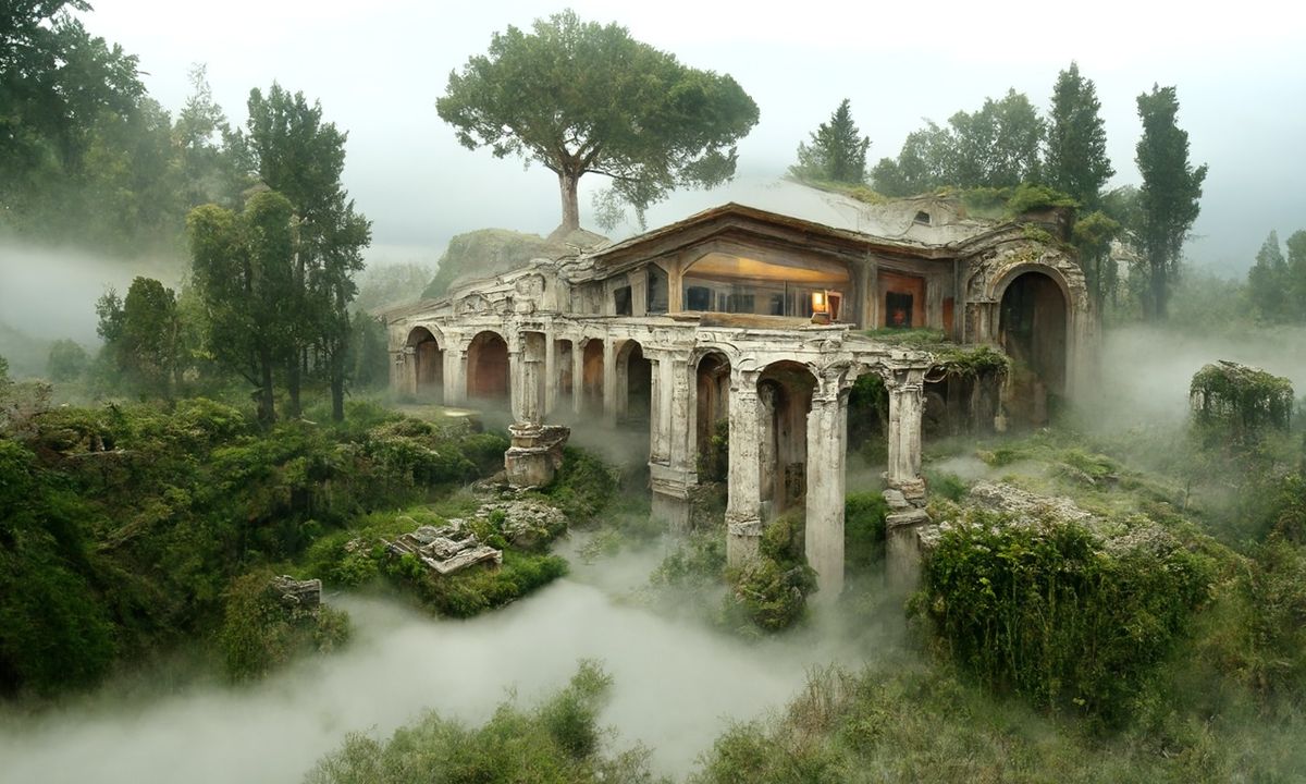
Disco Diffusion V4.1 Google Colab, Dall-E, Starryai – creating images with AI
Read more: Disco Diffusion V4.1 Google Colab, Dall-E, Starryai – creating images with AIDisco Diffusion (DD) is a Google Colab Notebook which leverages an AI Image generating technique called CLIP-Guided Diffusion to allow you to create compelling and beautiful images from just text inputs. Created by Somnai, augmented by Gandamu, and building on the work of RiversHaveWings, nshepperd, and many others.
Phone app: https://www.starryai.com/

docs.google.com/document/d/1l8s7uS2dGqjztYSjPpzlmXLjl5PM3IGkRWI3IiCuK7g

colab.research.google.com/drive/1sHfRn5Y0YKYKi1k-ifUSBFRNJ8_1sa39
Colab, or “Colaboratory”, allows you to write and execute Python in your browser, with
– Zero configuration required
– Access to GPUs free of charge
– Easy sharing


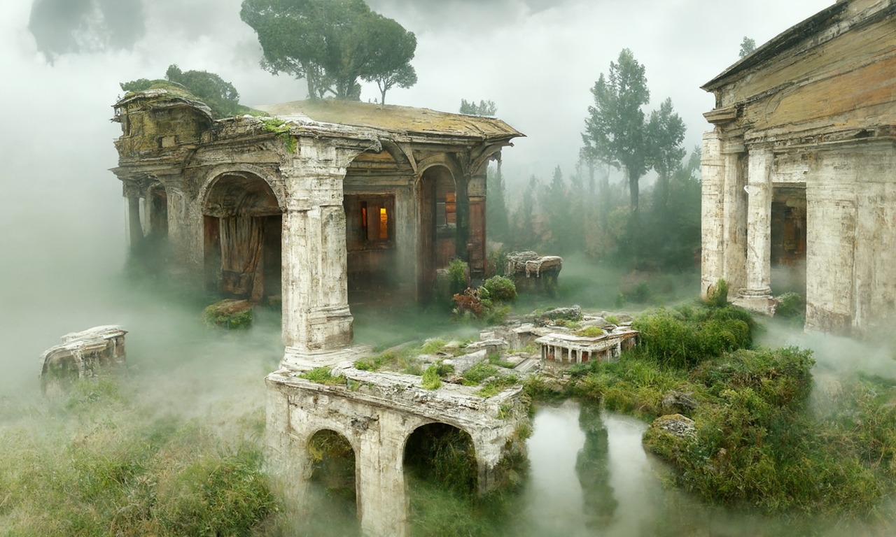
https://80.lv/articles/a-beautiful-roman-villa-made-with-disco-diffusion-5-2/
-
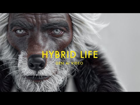
The Hybrids by Phil Langer – hyper-realistic AI-generated human animal portraits
Read more: The Hybrids by Phil Langer – hyper-realistic AI-generated human animal portraitshttps://www.reddit.com/r/aiArt/comments/1azepd6/hybrid_portraits_by_phil_langer/
https://www.thehybridportraits.com/
https://www.instagram.com/hybridportraits/


COLOR
-
Photography basics: Color Temperature and White Balance
Read more: Photography basics: Color Temperature and White Balance

Color Temperature of a light source describes the spectrum of light which is radiated from a theoretical “blackbody” (an ideal physical body that absorbs all radiation and incident light – neither reflecting it nor allowing it to pass through) with a given surface temperature.
https://en.wikipedia.org/wiki/Color_temperature
Or. Most simply it is a method of describing the color characteristics of light through a numerical value that corresponds to the color emitted by a light source, measured in degrees of Kelvin (K) on a scale from 1,000 to 10,000.
More accurately. The color temperature of a light source is the temperature of an ideal backbody that radiates light of comparable hue to that of the light source.
(more…) -
What Is The Resolution and view coverage Of The human Eye. And what distance is TV at best?
Read more: What Is The Resolution and view coverage Of The human Eye. And what distance is TV at best?
https://www.discovery.com/science/mexapixels-in-human-eye
About 576 megapixels for the entire field of view.
Consider a view in front of you that is 90 degrees by 90 degrees, like looking through an open window at a scene. The number of pixels would be:
90 degrees * 60 arc-minutes/degree * 1/0.3 * 90 * 60 * 1/0.3 = 324,000,000 pixels (324 megapixels).At any one moment, you actually do not perceive that many pixels, but your eye moves around the scene to see all the detail you want. But the human eye really sees a larger field of view, close to 180 degrees. Let’s be conservative and use 120 degrees for the field of view. Then we would see:
120 * 120 * 60 * 60 / (0.3 * 0.3) = 576 megapixels.
Or.
7 megapixels for the 2 degree focus arc… + 1 megapixel for the rest.
https://clarkvision.com/articles/eye-resolution.html
Details in the post
-
Victor Perez – The Color Management Handbook for Visual Effects Artists
Read more: Victor Perez – The Color Management Handbook for Visual Effects ArtistsDigital Color Principles, Color Management Fundamentals & ACES Workflows


LIGHTING
-
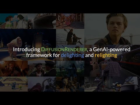
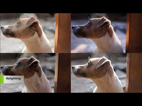
NVidia DiffusionRenderer – Neural Inverse and Forward Rendering with Video Diffusion Models. How NVIDIA reimagined relighting
Read more: NVidia DiffusionRenderer – Neural Inverse and Forward Rendering with Video Diffusion Models. How NVIDIA reimagined relightinghttps://www.fxguide.com/quicktakes/diffusing-reality-how-nvidia-reimagined-relighting/
https://research.nvidia.com/labs/toronto-ai/DiffusionRenderer/
-
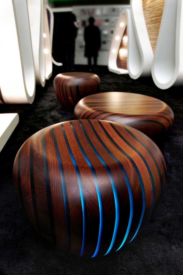
Composition – 5 tips for creating perfect cinematic lighting and making your work look stunning
Read more: Composition – 5 tips for creating perfect cinematic lighting and making your work look stunning
http://www.diyphotography.net/5-tips-creating-perfect-cinematic-lighting-making-work-look-stunning/
1. Learn the rules of lighting
2. Learn when to break the rules
3. Make your key light larger
4. Reverse keying
5. Always be backlighting
-
Composition – These are the basic lighting techniques you need to know for photography and film
Read more: Composition – These are the basic lighting techniques you need to know for photography and film
http://www.diyphotography.net/basic-lighting-techniques-need-know-photography-film/
Amongst the basic techniques, there’s…
1- Side lighting – Literally how it sounds, lighting a subject from the side when they’re faced toward you
2- Rembrandt lighting – Here the light is at around 45 degrees over from the front of the subject, raised and pointing down at 45 degrees
3- Back lighting – Again, how it sounds, lighting a subject from behind. This can help to add drama with silouettes
4- Rim lighting – This produces a light glowing outline around your subject
5- Key light – The main light source, and it’s not necessarily always the brightest light source
6- Fill light – This is used to fill in the shadows and provide detail that would otherwise be blackness
7- Cross lighting – Using two lights placed opposite from each other to light two subjects


COLLECTIONS
| Featured AI
| Design And Composition
| Explore posts
POPULAR SEARCHES
unreal | pipeline | virtual production | free | learn | photoshop | 360 | macro | google | nvidia | resolution | open source | hdri | real-time | photography basics | nuke
FEATURED POSTS
Social Links
DISCLAIMER – Links and images on this website may be protected by the respective owners’ copyright. All data submitted by users through this site shall be treated as freely available to share.
