To measure the contrast ratio you will need a light meter. The process starts with you measuring the main source of light, or the key light.
Get a reading from the brightest area on the face of your subject. Then, measure the area lit by the secondary light, or fill light. To make sense of what you have just measured you have to understand that the information you have just gathered is in F-stops, a measure of light. With each additional F-stop, for example going one stop from f/1.4 to f/2.0, you create a doubling of light. The reverse is also true; moving one stop from f/8.0 to f/5.6 results in a halving of the light.
this is the epic story of a group of talented digital artists trying to overcame daily technical challenges to achieve incredibly photorealistic projects of monsters and aliens
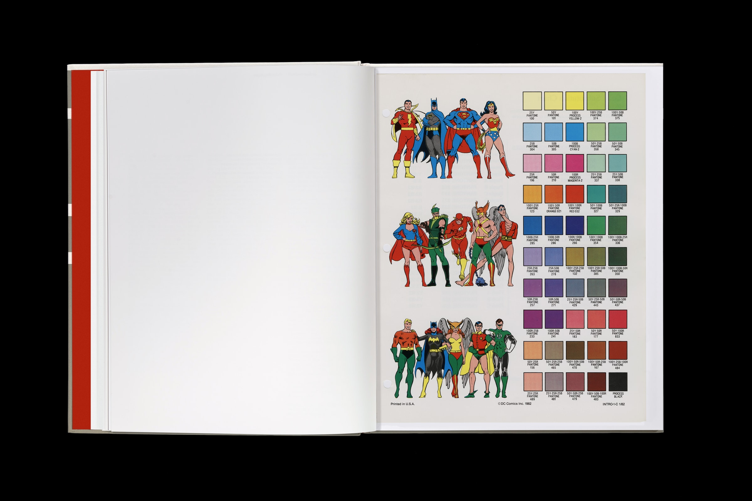
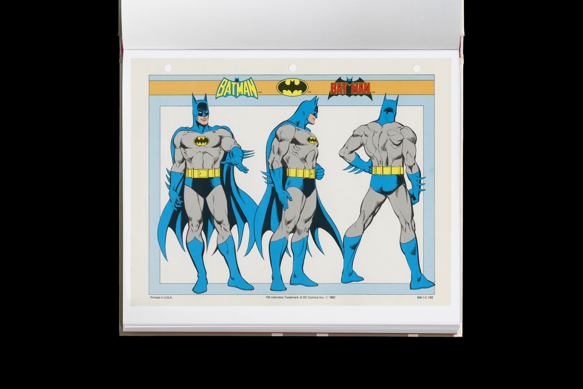
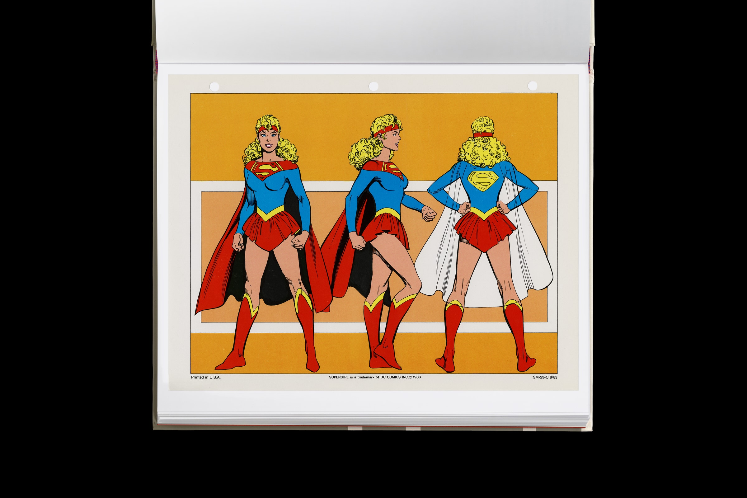
Reproduced from a rare original copy, the book features over 165 highly-detailed scans of the legendary art by José Luis García-López, with an introduction by Paul Levitz, former president of DC Comics.
The human eye perceives half scene brightness not as the linear 50% of the present energy (linear nature values) but as 18% of the overall brightness. We are biased to perceive more information in the dark and contrast areas. A Macbeth chart helps with calibrating back into a photographic capture into this “human perspective” of the world.
In photography, painting, and other visual arts, middle gray or middle grey is a tone that is perceptually about halfway between black and white on a lightness scale in photography and printing, it is typically defined as 18% reflectance in visible light
Light meters, cameras, and pictures are often calibrated using an 18% gray card[4][5][6] or a color reference card such as a ColorChecker. On the assumption that 18% is similar to the average reflectance of a scene, a grey card can be used to estimate the required exposure of the film.
ACES 2.0 is the second major release of the components that make up the ACES system. The most significant change is a new suite of rendering transforms whose design was informed by collected feedback and requests from users of ACES 1. The changes aim to improve the appearance of perceived artifacts and to complete previously unfinished components of the system, resulting in a more complete, robust, and consistent product.
Highlights of the key changes in ACES 2.0 are as follows:
New output transforms, including:
A less aggressive tone scale
More intuitive controls to create custom outputs to non-standard displays
Robust gamut mapping to improve perceptual uniformity
Improved performance of the inverse transforms
Enhanced AMF specification
An updated specification for ACES Transform IDs
OpenEXR compression recommendations
Enhanced tools for generating Input Transforms and recommended procedures for characterizing prosumer cameras
Look Transform Library
Expanded documentation
Rendering Transform
The most substantial change in ACES 2.0 is a complete redesign of the rendering transform.
ACES 2.0 was built as a unified system, rather than through piecemeal additions. Different deliverable outputs “match” better and making outputs to display setups other than the provided presets is intended to be user-driven. The rendering transforms are less likely to produce undesirable artifacts “out of the box”, which means less time can be spent fixing problematic images and more time making pictures look the way you want.
Key design goals
Improve consistency of tone scale and provide an easy to use parameter to allow for outputs between preset dynamic ranges
Minimize hue skews across exposure range in a region of same hue
Unify for structural consistency across transform type
Easy to use parameters to create outputs other than the presets
Robust gamut mapping to improve harsh clipping artifacts
Fill extents of output code value cube (where appropriate and expected)
Invertible – not necessarily reversible, but Output > ACES > Output round-trip should be possible
Accomplish all of the above while maintaining an acceptable “out-of-the box” rendering
In photography, exposure value (EV) is a number that represents a combination of a camera’s shutter speed and f-number, such that all combinations that yield the same exposure have the same EV (for any fixed scene luminance).
The EV concept was developed in an attempt to simplify choosing among combinations of equivalent camera settings. Although all camera settings with the same EV nominally give the same exposure, they do not necessarily give the same picture. EV is also used to indicate an interval on the photographic exposure scale. 1 EV corresponding to a standard power-of-2 exposure step, commonly referred to as a stop
EV 0 corresponds to an exposure time of 1 sec and a relative aperture of f/1.0. If the EV is known, it can be used to select combinations of exposure time and f-number.
Note EV does not equal to photographic exposure. Photographic Exposureis defined as how much light hits the camera’s sensor. It depends on the camera settings mainly aperture and shutter speed. Exposure value (known as EV) is a number that represents theexposure setting of the camera.
Thus, strictly, EV is not a measure of luminance (indirect or reflected exposure) or illuminance (incidentl exposure); rather, an EV corresponds to a luminance (or illuminance) for which a camera with a given ISO speed would use the indicated EV to obtain the nominally correct exposure. Nonetheless, it is common practice among photographic equipment manufacturers to express luminance in EV for ISO 100 speed, as when specifying metering range or autofocus sensitivity.
The exposure depends on two things: how much light gets through the lenses to the camera’s sensor and for how long the sensor is exposed. The former is a function of the aperture value while the latter is a function of the shutter speed. Exposure value is a number that represents this potential amount of light that could hit the sensor. It is important to understand that exposure value is a measure of how exposed the sensor is to light and not a measure of how much light actually hits the sensor. The exposure value is independent of how lit the scene is. For example a pair of aperture value and shutter speed represents the same exposure value both if the camera is used during a very bright day or during a dark night.
Each exposure value number represents all the possible shutter and aperture settings that result in the same exposure. Although the exposure value is the same for different combinations of aperture values and shutter speeds the resulting photo can be very different (the aperture controls the depth of field while shutter speed controls how much motion is captured).
EV 0.0 is defined as the exposure when setting the aperture to f-number 1.0 and the shutter speed to 1 second. All other exposure values are relative to that number. Exposure values are on a base two logarithmic scale. This means that every single step of EV – plus or minus 1 – represents the exposure (actual light that hits the sensor) being halved or doubled.
The human eye perceives half scene brightness not as the linear 50% of the present energy (linear nature values) but as 18% of the overall brightness. We are biased to perceive more information in the dark and contrast areas. A Macbeth chart helps with calibrating back into a photographic capture into this “human perspective” of the world.
In photography, painting, and other visual arts, middle gray or middle grey is a tone that is perceptually about halfway between black and white on a lightness scale in photography and printing, it is typically defined as 18% reflectance in visible light
Light meters, cameras, and pictures are often calibrated using an 18% gray card[4][5][6] or a color reference card such as a ColorChecker. On the assumption that 18% is similar to the average reflectance of a scene, a grey card can be used to estimate the required exposure of the film.
To measure the contrast ratio you will need a light meter. The process starts with you measuring the main source of light, or the key light.
Get a reading from the brightest area on the face of your subject. Then, measure the area lit by the secondary light, or fill light. To make sense of what you have just measured you have to understand that the information you have just gathered is in F-stops, a measure of light. With each additional F-stop, for example going one stop from f/1.4 to f/2.0, you create a doubling of light. The reverse is also true; moving one stop from f/8.0 to f/5.6 results in a halving of the light.
This 2025 I decided to start learning how to code, so I installed Visual Studio and I started looking into C++. After days of watching tutorials and guides about the basics of C++ and programming, I decided to make something physics-related. I started with a dot that fell to the ground and then I wanted to simulate gravitational attraction, so I made 2 circles attracting each other. I thought it was really cool to see something I made with code actually work, so I kept building on top of that small, basic program. And here we are after roughly 8 months of learning programming. This is Galaxy Engine, and it is a simulation software I have been making ever since I started my learning journey. It currently can simulate gravity, dark matter, galaxies, the Big Bang, temperature, fluid dynamics, breakable solids, planetary interactions, etc. The program can run many tens of thousands of particles in real time on the CPU thanks to the Barnes-Hut algorithm, mixed with Morton curves. It also includes its own PBR 2D path tracer with BVH optimizations. The path tracer can simulate a bunch of stuff like diffuse lighting, specular reflections, refraction, internal reflection, fresnel, emission, dispersion, roughness, IOR, nested IOR and more! I tried to make the path tracer closer to traditional 3D render engines like V-Ray. I honestly never imagined I would go this far with programming, and it has been an amazing learning experience so far. I think that mixing this knowledge with my 3D knowledge can unlock countless new possibilities. In case you are curious about Galaxy Engine, I made it completely free and Open-Source so that anyone can build and compile it locally! You can find the source code inGitHub
“Unless you have all the relevant spectral measurements, a colour rendition chart should not be used to perform colour-correction of camera imagery but only for white balancing and relative exposure adjustments.”
“Using a colour rendition chart for colour-correction might dramatically increase error if the scene light source spectrum is different from the illuminant used to compute the colour rendition chart’s reference values.”
“other factors make using a colour rendition chart unsuitable for camera calibration:
– Uncontrolled geometry of the colour rendition chart with the incident illumination and the camera.
– Unknown sample reflectances and ageing as the colour of the samples vary with time.
– Low samples count.
– Camera noise and flare.
– Etc…
“Those issues are well understood in the VFX industry, and when receiving plates, we almost exclusively use colour rendition charts to white balance and perform relative exposure adjustments, i.e. plate neutralisation.”
DISCLAIMER – Links and images on this website may be protected by the respective owners’ copyright. All data submitted by users through this site shall be treated as freely available to share.