


COMPOSITION


DESIGN


COLOR
-
What light is best to illuminate gems for resale
Read more: What light is best to illuminate gems for resalewww.palagems.com/gem-lighting2
Artificial light sources, not unlike the diverse phases of natural light, vary considerably in their properties. As a result, some lamps render an object’s color better than others do.
The most important criterion for assessing the color-rendering ability of any lamp is its spectral power distribution curve.
Natural daylight varies too much in strength and spectral composition to be taken seriously as a lighting standard for grading and dealing colored stones. For anything to be a standard, it must be constant in its properties, which natural light is not.
For dealers in particular to make the transition from natural light to an artificial light source, that source must offer:
1- A degree of illuminance at least as strong as the common phases of natural daylight.
2- Spectral properties identical or comparable to a phase of natural daylight.A source combining these two things makes gems appear much the same as when viewed under a given phase of natural light. From the viewpoint of many dealers, this corresponds to a naturalappearance.
The 6000° Kelvin xenon short-arc lamp appears closest to meeting the criteria for a standard light source. Besides the strong illuminance this lamp affords, its spectrum is very similar to CIE standard illuminants of similar color temperature.


-
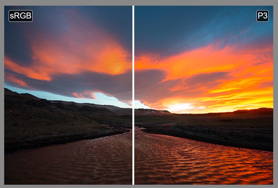
Colormaxxing – What if I told you that rgb(255, 0, 0) is not actually the reddest red you can have in your browser?
Read more: Colormaxxing – What if I told you that rgb(255, 0, 0) is not actually the reddest red you can have in your browser?https://karuna.dev/colormaxxing
https://webkit.org/blog-files/color-gamut/comparison.html
https://oklch.com/#70,0.1,197,100
-
PBR Color Reference List for Materials – by Grzegorz Baran
Read more: PBR Color Reference List for Materials – by Grzegorz Baran
“The list should be helpful for every material artist who work on PBR materials as it contains over 200 color values measured with PCE-RGB2 1002 Color Spectrometer device and presented in linear and sRGB (2.2) gamma space.
All color values, HUE and Saturation in this list come from measurements taken with PCE-RGB2 1002 Color Spectrometer device and are presented in linear and sRGB (2.2) gamma space (more info at the end of this video) I calculated Relative Luminance and Luminance values based on captured color using my own equation which takes color based luminance perception into consideration. Bare in mind that there is no ‘one’ color per substance as nothing in nature is even 100% uniform and any value in +/-10% range from these should be considered as correct one. Therefore this list should be always considered as a color reference for material’s albedos, not ulitimate and absolute truth.“


LIGHTING
-
3D Lighting Tutorial by Amaan Kram
Read more: 3D Lighting Tutorial by Amaan Kramhttp://www.amaanakram.com/lightingT/part1.htm
The goals of lighting in 3D computer graphics are more or less the same as those of real world lighting.
Lighting serves a basic function of bringing out, or pushing back the shapes of objects visible from the camera’s view.
It gives a two-dimensional image on the monitor an illusion of the third dimension-depth.But it does not just stop there. It gives an image its personality, its character. A scene lit in different ways can give a feeling of happiness, of sorrow, of fear etc., and it can do so in dramatic or subtle ways. Along with personality and character, lighting fills a scene with emotion that is directly transmitted to the viewer.
Trying to simulate a real environment in an artificial one can be a daunting task. But even if you make your 3D rendering look absolutely photo-realistic, it doesn’t guarantee that the image carries enough emotion to elicit a “wow” from the people viewing it.
Making 3D renderings photo-realistic can be hard. Putting deep emotions in them can be even harder. However, if you plan out your lighting strategy for the mood and emotion that you want your rendering to express, you make the process easier for yourself.
Each light source can be broken down in to 4 distinct components and analyzed accordingly.
· Intensity
· Direction
· Color
· SizeThe overall thrust of this writing is to produce photo-realistic images by applying good lighting techniques.

-
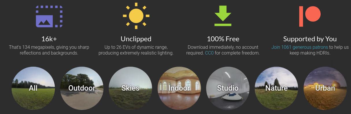
Free HDRI libraries
Read more: Free HDRI librariesnoahwitchell.com
http://www.noahwitchell.com/freebieslocationtextures.com
https://locationtextures.com/panoramas/maxroz.com
https://www.maxroz.com/hdri/listHDRI Haven
https://hdrihaven.com/Poly Haven
https://polyhaven.com/hdrisDomeble
https://www.domeble.com/IHDRI
https://www.ihdri.com/HDRMaps
https://hdrmaps.com/NoEmotionHdrs.net
http://noemotionhdrs.net/hdrday.htmlOpenFootage.net
https://www.openfootage.net/hdri-panorama/HDRI-hub
https://www.hdri-hub.com/hdrishop/hdri.zwischendrin
https://www.zwischendrin.com/en/browse/hdriLonger list here:
https://cgtricks.com/list-sites-free-hdri/
-
PTGui 13 beta adds control through a Patch Editor
Read more: PTGui 13 beta adds control through a Patch EditorAdditions:
- Patch Editor (PTGui Pro)
- DNG output
- Improved RAW / DNG handling
- JPEG 2000 support
- Performance improvements

-
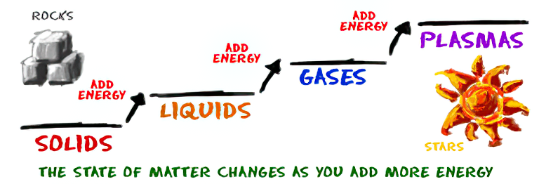
How are Energy and Matter the Same?
Read more: How are Energy and Matter the Same?www.turnerpublishing.com/blog/detail/everything-is-energy-everything-is-one-everything-is-possible/
www.universetoday.com/116615/how-are-energy-and-matter-the-same/
As Einstein showed us, light and matter and just aspects of the same thing. Matter is just frozen light. And light is matter on the move. Albert Einstein’s most famous equation says that energy and matter are two sides of the same coin. How does one become the other?
Relativity requires that the faster an object moves, the more mass it appears to have. This means that somehow part of the energy of the car’s motion appears to transform into mass. Hence the origin of Einstein’s equation. How does that happen? We don’t really know. We only know that it does.
Matter is 99.999999999999 percent empty space. Not only do the atom and solid matter consist mainly of empty space, it is the same in outer space
The quantum theory researchers discovered the answer: Not only do particles consist of energy, but so does the space between. This is the so-called zero-point energy. Therefore it is true: Everything consists of energy.
Energy is the basis of material reality. Every type of particle is conceived of as a quantum vibration in a field: Electrons are vibrations in electron fields, protons vibrate in a proton field, and so on. Everything is energy, and everything is connected to everything else through fields.
-
HDRI Resources
Read more: HDRI ResourcesText2Light
- https://www.cgtrader.com/free-3d-models/exterior/other/10-free-hdr-panoramas-created-with-text2light-zero-shot
- https://frozenburning.github.io/projects/text2light/
- https://github.com/FrozenBurning/Text2Light
Royalty free links
- https://locationtextures.com/panoramas/
- http://www.noahwitchell.com/freebies
- https://polyhaven.com/hdris
- https://hdrmaps.com/
- https://www.ihdri.com/
- https://hdrihaven.com/
- https://www.domeble.com/
- http://www.hdrlabs.com/sibl/archive.html
- https://www.hdri-hub.com/hdrishop/hdri
- http://noemotionhdrs.net/hdrevening.html
- https://www.openfootage.net/hdri-panorama/
- https://www.zwischendrin.com/en/browse/hdri
Nvidia GauGAN360
-
Fast, optimized ‘for’ pixel loops with OpenCV and Python to create tone mapped HDR images
Read more: Fast, optimized ‘for’ pixel loops with OpenCV and Python to create tone mapped HDR imageshttps://pyimagesearch.com/2017/08/28/fast-optimized-for-pixel-loops-with-opencv-and-python/
https://learnopencv.com/exposure-fusion-using-opencv-cpp-python/
Exposure Fusion is a method for combining images taken with different exposure settings into one image that looks like a tone mapped High Dynamic Range (HDR) image.


COLLECTIONS
| Featured AI
| Design And Composition
| Explore posts
POPULAR SEARCHES
unreal | pipeline | virtual production | free | learn | photoshop | 360 | macro | google | nvidia | resolution | open source | hdri | real-time | photography basics | nuke
FEATURED POSTS
-
Steven Stahlberg – Perception and Composition
-
Image rendering bit depth
-
sRGB vs REC709 – An introduction and FFmpeg implementations
-
Jesse Zumstein – Jobs in games
-
AI and the Law – Netflix : Using Generative AI in Content Production
-
AnimationXpress.com interviews Daniele Tosti for TheCgCareer.com channel
-
Photography basics: Solid Angle measures
-
Eddie Yoon – There’s a big misconception about AI creative
Social Links
DISCLAIMER – Links and images on this website may be protected by the respective owners’ copyright. All data submitted by users through this site shall be treated as freely available to share.
