


COMPOSITION
-
Composition – 5 tips for creating perfect cinematic lighting and making your work look stunning
Read more: Composition – 5 tips for creating perfect cinematic lighting and making your work look stunning
http://www.diyphotography.net/5-tips-creating-perfect-cinematic-lighting-making-work-look-stunning/
1. Learn the rules of lighting
2. Learn when to break the rules
3. Make your key light larger
4. Reverse keying
5. Always be backlighting
-
Photography basics: Depth of Field and composition
Read more: Photography basics: Depth of Field and compositionDepth of field is the range within which focusing is resolved in a photo.
Aperture has a huge affect on to the depth of field.
Changing the f-stops (f/#) of a lens will change aperture and as such the DOF.
f-stops are a just certain number which is telling you the size of the aperture. That’s how f-stop is related to aperture (and DOF).
If you increase f-stops, it will increase DOF, the area in focus (and decrease the aperture). On the other hand, decreasing the f-stop it will decrease DOF (and increase the aperture).
The red cone in the figure is an angular representation of the resolution of the system. Versus the dotted lines, which indicate the aperture coverage. Where the lines of the two cones intersect defines the total range of the depth of field.
This image explains why the longer the depth of field, the greater the range of clarity.


DESIGN
COLOR
-
Yasuharu YOSHIZAWA – Comparison of sRGB vs ACREScg in Nuke
Read more: Yasuharu YOSHIZAWA – Comparison of sRGB vs ACREScg in NukeAnswering the question that is often asked, “Do I need to use ACEScg to display an sRGB monitor in the end?” (Demonstration shown at an in-house seminar)
Comparison of scanlineRender output with extreme color lights on color charts with sRGB/ACREScg in color – OCIO -working space in NukeDownload the Nuke script:
-
Black Body color aka the Planckian Locus curve for white point eye perception
Read more: Black Body color aka the Planckian Locus curve for white point eye perceptionhttp://en.wikipedia.org/wiki/Black-body_radiation

Black-body radiation is the type of electromagnetic radiation within or surrounding a body in thermodynamic equilibrium with its environment, or emitted by a black body (an opaque and non-reflective body) held at constant, uniform temperature. The radiation has a specific spectrum and intensity that depends only on the temperature of the body.
A black-body at room temperature appears black, as most of the energy it radiates is infra-red and cannot be perceived by the human eye. At higher temperatures, black bodies glow with increasing intensity and colors that range from dull red to blindingly brilliant blue-white as the temperature increases.
The Black Body Ultraviolet Catastrophe Experiment
In photography, color temperature describes the spectrum of light which is radiated from a “blackbody” with that surface temperature. A blackbody is an object which absorbs all incident light — neither reflecting it nor allowing it to pass through.
The Sun closely approximates a black-body radiator. Another rough analogue of blackbody radiation in our day to day experience might be in heating a metal or stone: these are said to become “red hot” when they attain one temperature, and then “white hot” for even higher temperatures. Similarly, black bodies at different temperatures also have varying color temperatures of “white light.”
Despite its name, light which may appear white does not necessarily contain an even distribution of colors across the visible spectrum.
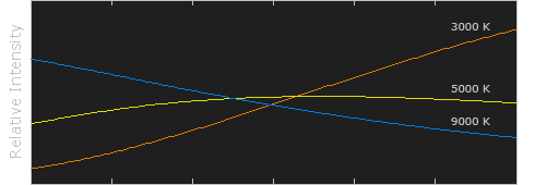
Although planets and stars are neither in thermal equilibrium with their surroundings nor perfect black bodies, black-body radiation is used as a first approximation for the energy they emit. Black holes are near-perfect black bodies, and it is believed that they emit black-body radiation (called Hawking radiation), with a temperature that depends on the mass of the hole.
-
THOMAS MANSENCAL – The Apparent Simplicity of RGB Rendering
Read more: THOMAS MANSENCAL – The Apparent Simplicity of RGB Rendering
https://thomasmansencal.substack.com/p/the-apparent-simplicity-of-rgb-rendering
The primary goal of physically-based rendering (PBR) is to create a simulation that accurately reproduces the imaging process of electro-magnetic spectrum radiation incident to an observer. This simulation should be indistinguishable from reality for a similar observer.
Because a camera is not sensitive to incident light the same way than a human observer, the images it captures are transformed to be colorimetric. A project might require infrared imaging simulation, a portion of the electro-magnetic spectrum that is invisible to us. Radically different observers might image the same scene but the act of observing does not change the intrinsic properties of the objects being imaged. Consequently, the physical modelling of the virtual scene should be independent of the observer.
-
What light is best to illuminate gems for resale
Read more: What light is best to illuminate gems for resalewww.palagems.com/gem-lighting2
Artificial light sources, not unlike the diverse phases of natural light, vary considerably in their properties. As a result, some lamps render an object’s color better than others do.
The most important criterion for assessing the color-rendering ability of any lamp is its spectral power distribution curve.
Natural daylight varies too much in strength and spectral composition to be taken seriously as a lighting standard for grading and dealing colored stones. For anything to be a standard, it must be constant in its properties, which natural light is not.
For dealers in particular to make the transition from natural light to an artificial light source, that source must offer:
1- A degree of illuminance at least as strong as the common phases of natural daylight.
2- Spectral properties identical or comparable to a phase of natural daylight.A source combining these two things makes gems appear much the same as when viewed under a given phase of natural light. From the viewpoint of many dealers, this corresponds to a naturalappearance.
The 6000° Kelvin xenon short-arc lamp appears closest to meeting the criteria for a standard light source. Besides the strong illuminance this lamp affords, its spectrum is very similar to CIE standard illuminants of similar color temperature.


-
Scene Referred vs Display Referred color workflows
Read more: Scene Referred vs Display Referred color workflowsDisplay Referred it is tied to the target hardware, as such it bakes color requirements into every type of media output request.
Scene Referred uses a common unified wide gamut and targeting audience through CDL and DI libraries instead.
So that color information stays untouched and only “transformed” as/when needed.


Sources:
– Victor Perez – Color Management Fundamentals & ACES Workflows in Nuke
– https://z-fx.nl/ColorspACES.pdf
– Wicus
-
The Maya civilization and the color blue
Read more: The Maya civilization and the color blueMaya blue is a highly unusual pigment because it is a mix of organic indigo and an inorganic clay mineral called palygorskite.
Echoing the color of an azure sky, the indelible pigment was used to accentuate everything from ceramics to human sacrifices in the Late Preclassic period (300 B.C. to A.D. 300).
A team of researchers led by Dean Arnold, an adjunct curator of anthropology at the Field Museum in Chicago, determined that the key to Maya blue was actually a sacred incense called copal.
By heating the mixture of indigo, copal and palygorskite over a fire, the Maya produced the unique pigment, he reported at the time.


LIGHTING
-
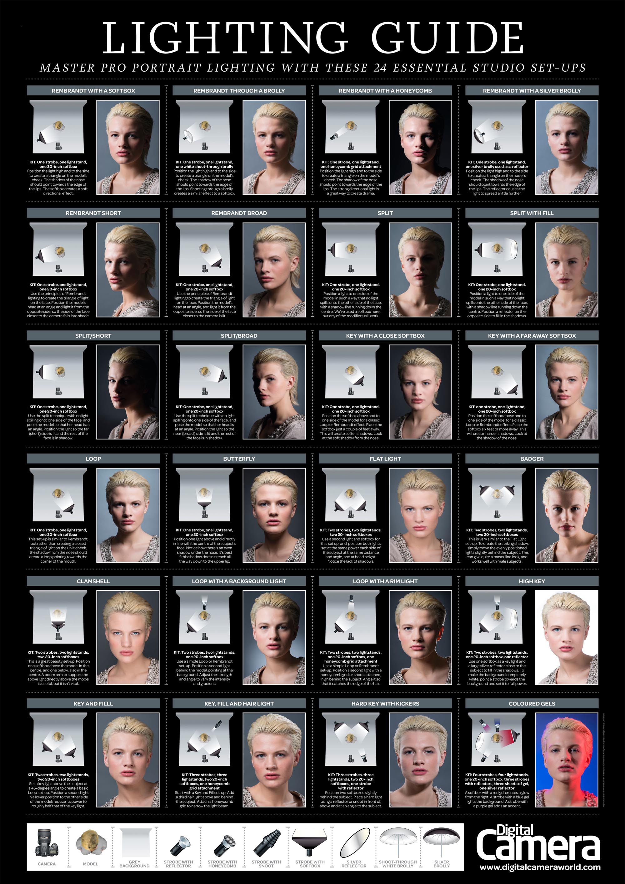
7 Easy Portrait Lighting Setups
Read more: 7 Easy Portrait Lighting Setups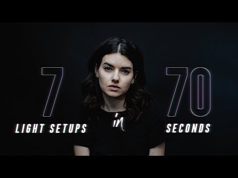
Butterfly
Loop
Rembrandt
Split
Rim
Broad
Short
-
PTGui 13 beta adds control through a Patch Editor
Read more: PTGui 13 beta adds control through a Patch EditorAdditions:
- Patch Editor (PTGui Pro)
- DNG output
- Improved RAW / DNG handling
- JPEG 2000 support
- Performance improvements


COLLECTIONS
| Featured AI
| Design And Composition
| Explore posts
POPULAR SEARCHES
unreal | pipeline | virtual production | free | learn | photoshop | 360 | macro | google | nvidia | resolution | open source | hdri | real-time | photography basics | nuke
FEATURED POSTS
-
Photography basics: Shutter angle and shutter speed and motion blur
-
Types of Film Lights and their efficiency – CRI, Color Temperature and Luminous Efficacy
-
Rec-2020 – TVs new color gamut standard used by Dolby Vision?
-
What Is The Resolution and view coverage Of The human Eye. And what distance is TV at best?
-
Web vs Printing or digital RGB vs CMYK
-
Convert 2D Images or Text to 3D Models
-
Ethan Roffler interviews CG Supervisor Daniele Tosti
-
Generative AI Glossary / AI Dictionary / AI Terminology
Social Links
DISCLAIMER – Links and images on this website may be protected by the respective owners’ copyright. All data submitted by users through this site shall be treated as freely available to share.
