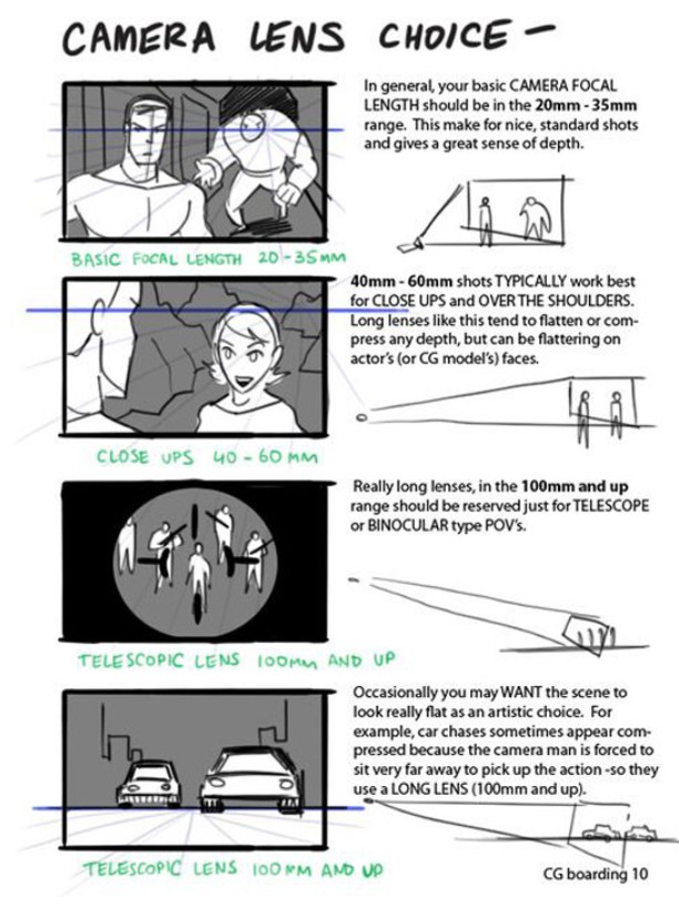
COMPOSITION
-
Composition – 5 tips for creating perfect cinematic lighting and making your work look stunning
Read more: Composition – 5 tips for creating perfect cinematic lighting and making your work look stunninghttp://www.diyphotography.net/5-tips-creating-perfect-cinematic-lighting-making-work-look-stunning/
1. Learn the rules of lighting
2. Learn when to break the rules
3. Make your key light larger
4. Reverse keying
5. Always be backlighting
DESIGN
COLOR
-
Photography basics: Lumens vs Candelas (candle) vs Lux vs FootCandle vs Watts vs Irradiance vs Illuminance
Read more: Photography basics: Lumens vs Candelas (candle) vs Lux vs FootCandle vs Watts vs Irradiance vs Illuminancehttps://www.translatorscafe.com/unit-converter/en-US/illumination/1-11/
The power output of a light source is measured using the unit of watts W. This is a direct measure to calculate how much power the light is going to drain from your socket and it is not relatable to the light brightness itself.
The amount of energy emitted from it per second. That energy comes out in a form of photons which we can crudely represent with rays of light coming out of the source. The higher the power the more rays emitted from the source in a unit of time.
Not all energy emitted is visible to the human eye, so we often rely on photometric measurements, which takes in account the sensitivity of human eye to different wavelenghts
Details in the post
(more…) -
The 7 key elements of brand identity design + 10 corporate identity examples
Read more: The 7 key elements of brand identity design + 10 corporate identity exampleswww.lucidpress.com/blog/the-7-key-elements-of-brand-identity-design
1. Clear brand purpose and positioning
2. Thorough market research
3. Likable brand personality
4. Memorable logo
5. Attractive color palette
6. Professional typography
7. On-brand supporting graphics
-
Virtual Production volumes study
Read more: Virtual Production volumes studyColor Fidelity in LED Volumes
https://theasc.com/articles/color-fidelity-in-led-volumesVirtual Production Glossary
https://vpglossary.com/What is Virtual Production – In depth analysis
https://www.leadingledtech.com/what-is-a-led-virtual-production-studio-in-depth-technical-analysis/A comparison of LED panels for use in Virtual Production:
Findings and recommendations
https://eprints.bournemouth.ac.uk/36826/1/LED_Comparison_White_Paper%281%29.pdf -
The Forbidden colors – Red-Green & Blue-Yellow: The Stunning Colors You Can’t See
Read more: The Forbidden colors – Red-Green & Blue-Yellow: The Stunning Colors You Can’t Seewww.livescience.com/17948-red-green-blue-yellow-stunning-colors.html
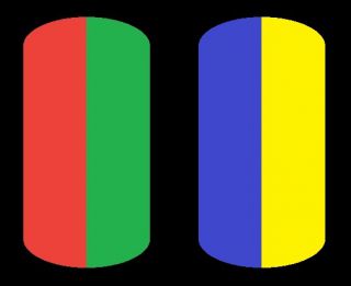
While the human eye has red, green, and blue-sensing cones, those cones are cross-wired in the retina to produce a luminance channel plus a red-green and a blue-yellow channel, and it’s data in that color space (known technically as “LAB”) that goes to the brain. That’s why we can’t perceive a reddish-green or a yellowish-blue, whereas such colors can be represented in the RGB color space used by digital cameras.
https://en.rockcontent.com/blog/the-use-of-yellow-in-data-design
The back of the retina is covered in light-sensitive neurons known as cone cells and rod cells. There are three types of cone cells, each sensitive to different ranges of light. These ranges overlap, but for convenience the cones are referred to as blue (short-wavelength), green (medium-wavelength), and red (long-wavelength). The rod cells are primarily used in low-light situations, so we’ll ignore those for now.
When light enters the eye and hits the cone cells, the cones get excited and send signals to the brain through the visual cortex. Different wavelengths of light excite different combinations of cones to varying levels, which generates our perception of color. You can see that the red cones are most sensitive to light, and the blue cones are least sensitive. The sensitivity of green and red cones overlaps for most of the visible spectrum.
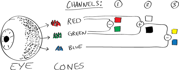
Here’s how your brain takes the signals of light intensity from the cones and turns it into color information. To see red or green, your brain finds the difference between the levels of excitement in your red and green cones. This is the red-green channel.
To get “brightness,” your brain combines the excitement of your red and green cones. This creates the luminance, or black-white, channel. To see yellow or blue, your brain then finds the difference between this luminance signal and the excitement of your blue cones. This is the yellow-blue channel.
From the calculations made in the brain along those three channels, we get four basic colors: blue, green, yellow, and red. Seeing blue is what you experience when low-wavelength light excites the blue cones more than the green and red.
Seeing green happens when light excites the green cones more than the red cones. Seeing red happens when only the red cones are excited by high-wavelength light.
Here’s where it gets interesting. Seeing yellow is what happens when BOTH the green AND red cones are highly excited near their peak sensitivity. This is the biggest collective excitement that your cones ever have, aside from seeing pure white.
Notice that yellow occurs at peak intensity in the graph to the right. Further, the lens and cornea of the eye happen to block shorter wavelengths, reducing sensitivity to blue and violet light.
-
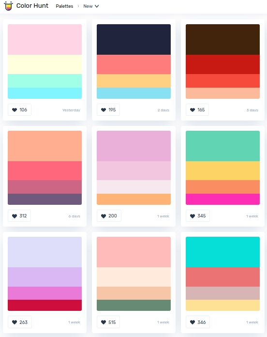
colorhunt.co
Read more: colorhunt.coColor Hunt is a free and open platform for color inspiration with thousands of trendy hand-picked color palettes.
-
sRGB vs REC709 – An introduction and FFmpeg implementations
Read more: sRGB vs REC709 – An introduction and FFmpeg implementations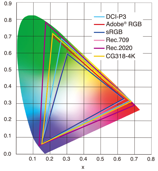
1. Basic Comparison
- What they are
- sRGB: A standard “web”/computer-display RGB color space defined by IEC 61966-2-1. It’s used for most monitors, cameras, printers, and the vast majority of images on the Internet.
- Rec. 709: An HD-video color space defined by ITU-R BT.709. It’s the go-to standard for HDTV broadcasts, Blu-ray discs, and professional video pipelines.
- Why they exist
- sRGB: Ensures consistent colors across different consumer devices (PCs, phones, webcams).
- Rec. 709: Ensures consistent colors across video production and playback chains (cameras → editing → broadcast → TV).
- What you’ll see
- On your desktop or phone, images tagged sRGB will look “right” without extra tweaking.
- On an HDTV or video-editing timeline, footage tagged Rec. 709 will display accurate contrast and hue on broadcast-grade monitors.
2. Digging Deeper
Feature sRGB Rec. 709 White point D65 (6504 K), same for both D65 (6504 K) Primaries (x,y) R: (0.640, 0.330) G: (0.300, 0.600) B: (0.150, 0.060) R: (0.640, 0.330) G: (0.300, 0.600) B: (0.150, 0.060) Gamut size Identical triangle on CIE 1931 chart Identical to sRGB Gamma / transfer Piecewise curve: approximate 2.2 with linear toe Pure power-law γ≈2.4 (often approximated as 2.2 in practice) Matrix coefficients N/A (pure RGB usage) Y = 0.2126 R + 0.7152 G + 0.0722 B (Rec. 709 matrix) Typical bit-depth 8-bit/channel (with 16-bit variants) 8-bit/channel (10-bit for professional video) Usage metadata Tagged as “sRGB” in image files (PNG, JPEG, etc.) Tagged as “bt709” in video containers (MP4, MOV) Color range Full-range RGB (0–255) Studio-range Y′CbCr (Y′ [16–235], Cb/Cr [16–240])
Why the Small Differences Matter
(more…) - What they are
-
FXGuide – ACES 2.0 with ILM’s Alex Fry
Read more: FXGuide – ACES 2.0 with ILM’s Alex Fryhttps://draftdocs.acescentral.com/background/whats-new/
ACES 2.0 is the second major release of the components that make up the ACES system. The most significant change is a new suite of rendering transforms whose design was informed by collected feedback and requests from users of ACES 1. The changes aim to improve the appearance of perceived artifacts and to complete previously unfinished components of the system, resulting in a more complete, robust, and consistent product.
Highlights of the key changes in ACES 2.0 are as follows:
- New output transforms, including:
- A less aggressive tone scale
- More intuitive controls to create custom outputs to non-standard displays
- Robust gamut mapping to improve perceptual uniformity
- Improved performance of the inverse transforms
- Enhanced AMF specification
- An updated specification for ACES Transform IDs
- OpenEXR compression recommendations
- Enhanced tools for generating Input Transforms and recommended procedures for characterizing prosumer cameras
- Look Transform Library
- Expanded documentation
Rendering Transform
The most substantial change in ACES 2.0 is a complete redesign of the rendering transform.
ACES 2.0 was built as a unified system, rather than through piecemeal additions. Different deliverable outputs “match” better and making outputs to display setups other than the provided presets is intended to be user-driven. The rendering transforms are less likely to produce undesirable artifacts “out of the box”, which means less time can be spent fixing problematic images and more time making pictures look the way you want.
Key design goals
- Improve consistency of tone scale and provide an easy to use parameter to allow for outputs between preset dynamic ranges
- Minimize hue skews across exposure range in a region of same hue
- Unify for structural consistency across transform type
- Easy to use parameters to create outputs other than the presets
- Robust gamut mapping to improve harsh clipping artifacts
- Fill extents of output code value cube (where appropriate and expected)
- Invertible – not necessarily reversible, but Output > ACES > Output round-trip should be possible
- Accomplish all of the above while maintaining an acceptable “out-of-the box” rendering
- New output transforms, including:
-
PBR Color Reference List for Materials – by Grzegorz Baran
Read more: PBR Color Reference List for Materials – by Grzegorz Baran“The list should be helpful for every material artist who work on PBR materials as it contains over 200 color values measured with PCE-RGB2 1002 Color Spectrometer device and presented in linear and sRGB (2.2) gamma space.
All color values, HUE and Saturation in this list come from measurements taken with PCE-RGB2 1002 Color Spectrometer device and are presented in linear and sRGB (2.2) gamma space (more info at the end of this video) I calculated Relative Luminance and Luminance values based on captured color using my own equation which takes color based luminance perception into consideration. Bare in mind that there is no ‘one’ color per substance as nothing in nature is even 100% uniform and any value in +/-10% range from these should be considered as correct one. Therefore this list should be always considered as a color reference for material’s albedos, not ulitimate and absolute truth.“
-
Capturing the world in HDR for real time projects – Call of Duty: Advanced Warfare
Read more: Capturing the world in HDR for real time projects – Call of Duty: Advanced WarfareReal-World Measurements for Call of Duty: Advanced Warfare
www.activision.com/cdn/research/Real_World_Measurements_for_Call_of_Duty_Advanced_Warfare.pdf
Local version
Real_World_Measurements_for_Call_of_Duty_Advanced_Warfare.pdf
LIGHTING
-
Practical Aspects of Spectral Data and LEDs in Digital Content Production and Virtual Production – SIGGRAPH 2022
Read more: Practical Aspects of Spectral Data and LEDs in Digital Content Production and Virtual Production – SIGGRAPH 2022Comparison to the commercial side
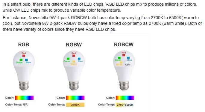
https://www.ecolorled.com/blog/detail/what-is-rgb-rgbw-rgbic-strip-lights
RGBW (RGB + White) LED strip uses a 4-in-1 LED chip made up of red, green, blue, and white.
RGBWW (RGB + White + Warm White) LED strip uses either a 5-in-1 LED chip with red, green, blue, white, and warm white for color mixing. The only difference between RGBW and RGBWW is the intensity of the white color. The term RGBCCT consists of RGB and CCT. CCT (Correlated Color Temperature) means that the color temperature of the led strip light can be adjusted to change between warm white and white. Thus, RGBWW strip light is another name of RGBCCT strip.
RGBCW is the acronym for Red, Green, Blue, Cold, and Warm. These 5-in-1 chips are used in supper bright smart LED lighting products
-
Light and Matter : The 2018 theory of Physically-Based Rendering and Shading by Allegorithmic
Read more: Light and Matter : The 2018 theory of Physically-Based Rendering and Shading by Allegorithmicacademy.substance3d.com/courses/the-pbr-guide-part-1
academy.substance3d.com/courses/the-pbr-guide-part-2
Local copy:
COLLECTIONS
| Featured AI
| Design And Composition
| Explore posts
POPULAR SEARCHES
unreal | pipeline | virtual production | free | learn | photoshop | 360 | macro | google | nvidia | resolution | open source | hdri | real-time | photography basics | nuke
FEATURED POSTS
-
Rec-2020 – TVs new color gamut standard used by Dolby Vision?
-
PixelSham – Introduction to Python 2022
-
Top 3D Printing Website Resources
-
Decart AI Mirage – The first ever World Transformation Model – turning any video, game, or camera feed into a new digital world, in real time
-
ComfyUI FLOAT – A container for FLOAT Generative Motion Latent Flow Matching for Audio-driven Talking Portrait – lip sync
-
How do LLMs like ChatGPT (Generative Pre-Trained Transformer) work? Explained by Deep-Fake Ryan Gosling
-
SourceTree vs Github Desktop – Which one to use
-
What Is The Resolution and view coverage Of The human Eye. And what distance is TV at best?
Social Links
DISCLAIMER – Links and images on this website may be protected by the respective owners’ copyright. All data submitted by users through this site shall be treated as freely available to share.


