To measure the contrast ratio you will need a light meter. The process starts with you measuring the main source of light, or the key light.
Get a reading from the brightest area on the face of your subject. Then, measure the area lit by the secondary light, or fill light. To make sense of what you have just measured you have to understand that the information you have just gathered is in F-stops, a measure of light. With each additional F-stop, for example going one stop from f/1.4 to f/2.0, you create a doubling of light. The reverse is also true; moving one stop from f/8.0 to f/5.6 results in a halving of the light.
” In this video, I utilized artificial intelligence to generate an animated music video for the song Canvas by Resonate. This tool allows anyone to generate beautiful images using only text as the input. My question was, what if I used song lyrics as input to the AI, can I make perfect music synchronized videos automatically with the push of a button? Let me know how you think the AI did in this visual interpretation of the song.
After getting caught up in the excitement around DALL·E2 (latest and greatest AI system, it’s INSANE), I searched for any way I could use similar image generation for music synchronization. Since DALL·E2 is not available to the public yet, my search led me to VQGAN + CLIP (Vector Quantized Generative Adversarial Network and Contrastive Language–Image Pre-training), before settling more specifically on Disco Diffusion V5.2 Turbo. If you don’t know what any of these words or acronyms mean, don’t worry, I was just as confused when I first started learning about this technology. I believe we’re reaching a turning point where entire industries are about to shift in reaction to this new process (which is essentially magic!).
Black-body radiation is the type of electromagnetic radiation within or surrounding a body in thermodynamic equilibrium with its environment, or emitted by a black body (an opaque and non-reflective body) held at constant, uniform temperature. The radiation has a specific spectrum and intensity that depends only on the temperature of the body.
A black-body at room temperature appears black, as most of the energy it radiates is infra-red and cannot be perceived by the human eye. At higher temperatures, black bodies glow with increasing intensity and colors that range from dull red to blindingly brilliant blue-white as the temperature increases.
The dynamic range is a ratio between the maximum and minimum values of a physical measurement. Its definition depends on what the dynamic range refers to.
For a scene: Dynamic range is the ratio between the brightest and darkest parts of the scene.
For a camera: Dynamic range is the ratio of saturation to noise. More specifically, the ratio of the intensity that just saturates the camera to the intensity that just lifts the camera response one standard deviation above camera noise.
For a display: Dynamic range is the ratio between the maximum and minimum intensities emitted from the screen.
The Dynamic Range of real-world scenes can be quite high — ratios of 100,000:1 are common in the natural world. An HDR (High Dynamic Range) image stores pixel values that span the whole tonal range of real-world scenes. Therefore, an HDR image is encoded in a format that allows the largest range of values, e.g. floating-point values stored with 32 bits per color channel. Another characteristics of an HDR image is that it stores linear values. This means that the value of a pixel from an HDR image is proportional to the amount of light measured by the camera.
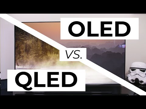
For TVs HDR is great, but it’s not the only new TV feature worth discussing.
Supported by LG, Philips, Panasonic and Sony sell the OLED system TVs. OLED stands for “organic light emitting diode.” It is a fundamentally different technology from LCD, the major type of TV today. OLED is “emissive,” meaning the pixels emit their own light.
Samsung is branding its best TVs with a new acronym: “QLED” QLED (according to Samsung) stands for “quantum dot LED TV.” It is a variation of the common LED LCD, adding a quantum dot film to the LCD “sandwich.” QLED, like LCD, is, in its current form, “transmissive” and relies on an LED backlight.
OLED is the only technology capable of absolute blacks and extremely bright whites on a per-pixel basis. LCD definitely can’t do that, and even the vaunted, beloved, dearly departed plasma couldn’t do absolute blacks.
QLED, as an improvement over OLED, significantly improves the picture quality. QLED can produce an even wider range of colors than OLED, which says something about this new tech. QLED is also known to produce up to 40% higher luminance efficiency than OLED technology. Further, many tests conclude that QLED is far more efficient in terms of power consumption than its predecessor, OLED.
DISCLAIMER – Links and images on this website may be protected by the respective owners’ copyright. All data submitted by users through this site shall be treated as freely available to share.