


COMPOSITION
-
SlowMoVideo – How to make a slow motion shot with the open source program
Read more: SlowMoVideo – How to make a slow motion shot with the open source programhttp://slowmovideo.granjow.net/
slowmoVideo is an OpenSource program that creates slow-motion videos from your footage.
Slow motion cinematography is the result of playing back frames for a longer duration than they were exposed. For example, if you expose 240 frames of film in one second, then play them back at 24 fps, the resulting movie is 10 times longer (slower) than the original filmed event….
Film cameras are relatively simple mechanical devices that allow you to crank up the speed to whatever rate the shutter and pull-down mechanism allow. Some film cameras can operate at 2,500 fps or higher (although film shot in these cameras often needs some readjustment in postproduction). Video, on the other hand, is always captured, recorded, and played back at a fixed rate, with a current limit around 60fps. This makes extreme slow motion effects harder to achieve (and less elegant) on video, because slowing down the video results in each frame held still on the screen for a long time, whereas with high-frame-rate film there are plenty of frames to fill the longer durations of time. On video, the slow motion effect is more like a slide show than smooth, continuous motion.
One obvious solution is to shoot film at high speed, then transfer it to video (a case where film still has a clear advantage, sorry George). Another possibility is to cross dissolve or blur from one frame to the next. This adds a smooth transition from one still frame to the next. The blur reduces the sharpness of the image, and compared to slowing down images shot at a high frame rate, this is somewhat of a cheat. However, there isn’t much you can do about it until video can be recorded at much higher rates. Of course, many film cameras can’t shoot at high frame rates either, so the whole super-slow-motion endeavor is somewhat specialized no matter what medium you are using. (There are some high speed digital cameras available now that allow you to capture lots of digital frames directly to your computer, so technology is starting to catch up with film. However, this feature isn’t going to appear in consumer camcorders any time soon.)
-
Types of Film Lights and their efficiency – CRI, Color Temperature and Luminous Efficacy
Read more: Types of Film Lights and their efficiency – CRI, Color Temperature and Luminous Efficacynofilmschool.com/types-of-film-lights
“Not every light performs the same way. Lights and lighting are tricky to handle. You have to plan for every circumstance. But the good news is, lighting can be adjusted. Let’s look at different factors that affect lighting in every scene you shoot. “
Use CRI, Luminous Efficacy and color temperature controls to match your needs.
Color Temperature
Color temperature describes the “color” of white light by a light source radiated by a perfect black body at a given temperature measured in degrees Kelvinhttps://www.pixelsham.com/2019/10/18/color-temperature/
CRI
“The Color Rendering Index is a measurement of how faithfully a light source reveals the colors of whatever it illuminates, it describes the ability of a light source to reveal the color of an object, as compared to the color a natural light source would provide. The highest possible CRI is 100. A CRI of 100 generally refers to a perfect black body, like a tungsten light source or the sun. “https://www.studiobinder.com/blog/what-is-color-rendering-index
(more…)


DESIGN


COLOR
-
Composition – cinematography Cheat Sheet
Read more: Composition – cinematography Cheat Sheet
Where is our eye attracted first? Why?
Size. Focus. Lighting. Color.
Size. Mr. White (Harvey Keitel) on the right.
Focus. He’s one of the two objects in focus.
Lighting. Mr. White is large and in focus and Mr. Pink (Steve Buscemi) is highlighted by
a shaft of light.
Color. Both are black and white but the read on Mr. White’s shirt now really stands out.
(more…)
What type of lighting? -
3D Lighting Tutorial by Amaan Kram
Read more: 3D Lighting Tutorial by Amaan Kramhttp://www.amaanakram.com/lightingT/part1.htm
The goals of lighting in 3D computer graphics are more or less the same as those of real world lighting.
Lighting serves a basic function of bringing out, or pushing back the shapes of objects visible from the camera’s view.
It gives a two-dimensional image on the monitor an illusion of the third dimension-depth.But it does not just stop there. It gives an image its personality, its character. A scene lit in different ways can give a feeling of happiness, of sorrow, of fear etc., and it can do so in dramatic or subtle ways. Along with personality and character, lighting fills a scene with emotion that is directly transmitted to the viewer.
Trying to simulate a real environment in an artificial one can be a daunting task. But even if you make your 3D rendering look absolutely photo-realistic, it doesn’t guarantee that the image carries enough emotion to elicit a “wow” from the people viewing it.
Making 3D renderings photo-realistic can be hard. Putting deep emotions in them can be even harder. However, if you plan out your lighting strategy for the mood and emotion that you want your rendering to express, you make the process easier for yourself.
Each light source can be broken down in to 4 distinct components and analyzed accordingly.
· Intensity
· Direction
· Color
· SizeThe overall thrust of this writing is to produce photo-realistic images by applying good lighting techniques.

-
OLED vs QLED – What TV is better?
Read more: OLED vs QLED – What TV is better?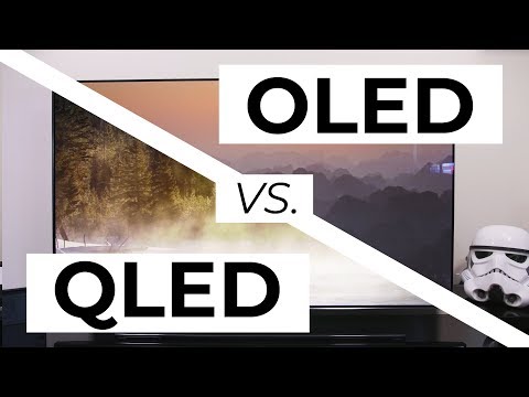
Supported by LG, Philips, Panasonic and Sony sell the OLED system TVs.
OLED stands for “organic light emitting diode.”
It is a fundamentally different technology from LCD, the major type of TV today.
OLED is “emissive,” meaning the pixels emit their own light.Samsung is branding its best TVs with a new acronym: “QLED”
QLED (according to Samsung) stands for “quantum dot LED TV.”
It is a variation of the common LED LCD, adding a quantum dot film to the LCD “sandwich.”
QLED, like LCD, is, in its current form, “transmissive” and relies on an LED backlight.OLED is the only technology capable of absolute blacks and extremely bright whites on a per-pixel basis. LCD definitely can’t do that, and even the vaunted, beloved, dearly departed plasma couldn’t do absolute blacks.
QLED, as an improvement over OLED, significantly improves the picture quality. QLED can produce an even wider range of colors than OLED, which says something about this new tech. QLED is also known to produce up to 40% higher luminance efficiency than OLED technology. Further, many tests conclude that QLED is far more efficient in terms of power consumption than its predecessor, OLED.
(more…) -
The 7 key elements of brand identity design + 10 corporate identity examples
Read more: The 7 key elements of brand identity design + 10 corporate identity exampleswww.lucidpress.com/blog/the-7-key-elements-of-brand-identity-design
1. Clear brand purpose and positioning
2. Thorough market research
3. Likable brand personality
4. Memorable logo
5. Attractive color palette
6. Professional typography
7. On-brand supporting graphics

-
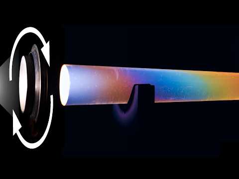
Polarised vs unpolarized filtering
Read more: Polarised vs unpolarized filteringA light wave that is vibrating in more than one plane is referred to as unpolarized light. …
Polarized light waves are light waves in which the vibrations occur in a single plane. The process of transforming unpolarized light into polarized light is known as polarization.

en.wikipedia.org/wiki/Polarizing_filter_(photography)
The most common use of polarized technology is to reduce lighting complexity on the subject.
(more…)
Details such as glare and hard edges are not removed, but greatly reduced. -
Pattern generators
Read more: Pattern generatorshttp://qrohlf.com/trianglify-generator/
https://halftonepro.com/app/polygons#
https://mattdesl.svbtle.com/generative-art-with-nodejs-and-canvas
https://www.patterncooler.com/
http://permadi.com/java/spaint/spaint.html
https://dribbble.com/shots/1847313-Kaleidoscope-Generator-PSD
http://eskimoblood.github.io/gerstnerizer/
http://www.stripegenerator.com/
http://btmills.github.io/geopattern/geopattern.html
http://fractalarchitect.net/FA4-Random-Generator.html
https://sciencevsmagic.net/fractal/#0605,0000,3,2,0,1,2
https://sites.google.com/site/mandelbulber/home


LIGHTING
-
Arto T. – A workflow for creating photorealistic, equirectangular 360° panoramas in ComfyUI using Flux
Read more: Arto T. – A workflow for creating photorealistic, equirectangular 360° panoramas in ComfyUI using Fluxhttps://civitai.com/models/735980/flux-equirectangular-360-panorama
https://civitai.com/models/745010?modelVersionId=833115
The trigger phrase is “equirectangular 360 degree panorama”. I would avoid saying “spherical projection” since that tends to result in non-equirectangular spherical images.
Image resolution should always be a 2:1 aspect ratio. 1024 x 512 or 1408 x 704 work quite well and were used in the training data. 2048 x 1024 also works.
I suggest using a weight of 0.5 – 1.5. If you are having issues with the image generating too flat instead of having the necessary spherical distortion, try increasing the weight above 1, though this could negatively impact small details of the image. For Flux guidance, I recommend a value of about 2.5 for realistic scenes.
8-bit output at the moment


-
Outpost VFX lighting tips
Read more: Outpost VFX lighting tipswww.outpost-vfx.com/en/news/18-pro-tips-and-tricks-for-lighting
Get as much information regarding your plate lighting as possible
- Always use a reference
- Replicate what is happening in real life
- Invest into a solid HDRI
- Start Simple
- Observe real world lighting, photography and cinematography
- Don’t neglect the theory
- Learn the difference between realism and photo-realism.
- Keep your scenes organised

-
Christopher Butler – Understanding the Eye-Mind Connection – Vision is a mental process
Read more: Christopher Butler – Understanding the Eye-Mind Connection – Vision is a mental processhttps://www.chrbutler.com/understanding-the-eye-mind-connection
The intricate relationship between the eyes and the brain, often termed the eye-mind connection, reveals that vision is predominantly a cognitive process. This understanding has profound implications for fields such as design, where capturing and maintaining attention is paramount. This essay delves into the nuances of visual perception, the brain’s role in interpreting visual data, and how this knowledge can be applied to effective design strategies.
This cognitive aspect of vision is evident in phenomena such as optical illusions, where the brain interprets visual information in a way that contradicts physical reality. These illusions underscore that what we “see” is not merely a direct recording of the external world but a constructed experience shaped by cognitive processes.
Understanding the cognitive nature of vision is crucial for effective design. Designers must consider how the brain processes visual information to create compelling and engaging visuals. This involves several key principles:
- Attention and Engagement
- Visual Hierarchy
- Cognitive Load Management
- Context and Meaning

-
Open Source Nvidia Omniverse
Read more: Open Source Nvidia Omniverseblogs.nvidia.com/blog/2019/03/18/omniverse-collaboration-platform/
developer.nvidia.com/nvidia-omniverse
An open, Interactive 3D Design Collaboration Platform for Multi-Tool Workflows to simplify studio workflows for real-time graphics.
It supports Pixar’s Universal Scene Description technology for exchanging information about modeling, shading, animation, lighting, visual effects and rendering across multiple applications.
It also supports NVIDIA’s Material Definition Language, which allows artists to exchange information about surface materials across multiple tools.
With Omniverse, artists can see live updates made by other artists working in different applications. They can also see changes reflected in multiple tools at the same time.
For example an artist using Maya with a portal to Omniverse can collaborate with another artist using UE4 and both will see live updates of each others’ changes in their application.


COLLECTIONS
| Featured AI
| Design And Composition
| Explore posts
POPULAR SEARCHES
unreal | pipeline | virtual production | free | learn | photoshop | 360 | macro | google | nvidia | resolution | open source | hdri | real-time | photography basics | nuke
FEATURED POSTS
-
Principles of Animation with Alan Becker, Dermot OConnor and Shaun Keenan
-
RawTherapee – a free, open source, cross-platform raw image and HDRi processing program
-
Convert 2D Images or Text to 3D Models
-
Top 3D Printing Website Resources
-
How to paint a boardgame miniatures
-
AI and the Law – Netflix : Using Generative AI in Content Production
-
Emmanuel Tsekleves – Writing Research Papers
-
Photography basics: Color Temperature and White Balance
Social Links
DISCLAIMER – Links and images on this website may be protected by the respective owners’ copyright. All data submitted by users through this site shall be treated as freely available to share.
