Björn Ottosson proposed OKlch in 2020 to create a color space that can closely mimic how color is perceived by the human eye, predicting perceived lightness, chroma, and hue.
The OK in OKLCH stands for Optimal Color.
L: Lightness (the perceived brightness of the color)
C: Chroma (the intensity or saturation of the color)
H: Hue (the actual color, such as red, blue, green, etc.)
The Manuka rendering architecture has been designed in the spirit of the classic reyes rendering architecture. In its core, reyes is based on stochastic rasterisation of micropolygons, facilitating depth of field, motion blur, high geometric complexity,and programmable shading.
This is commonly achieved with Monte Carlo path tracing, using a paradigm often called shade-on-hit, in which the renderer alternates tracing rays with running shaders on the various ray hits. The shaders take the role of generating the inputs of the local material structure which is then used bypath sampling logic to evaluate contributions and to inform what further rays to cast through the scene.
Over the years, however, the expectations have risen substantially when it comes to image quality. Computing pictures which are indistinguishable from real footage requires accurate simulation of light transport, which is most often performed using some variant of Monte Carlo path tracing. Unfortunately this paradigm requires random memory accesses to the whole scene and does not lend itself well to a rasterisation approach at all.
Manuka is both a uni-directional and bidirectional path tracer and encompasses multiple importance sampling (MIS). Interestingly, and importantly for production character skin work, it is the first major production renderer to incorporate spectral MIS in the form of a new ‘Hero Spectral Sampling’ technique, which was recently published at Eurographics Symposium on Rendering 2014.
Manuka propose a shade-before-hit paradigm in-stead and minimise I/O strain (and some memory costs) on the system, leveraging locality of reference by running pattern generation shaders before we execute light transport simulation by path sampling, “compressing” any bvh structure as needed, and as such also limiting duplication of source data.
The difference with reyes is that instead of baking colors into the geometry like in Reyes, manuka bakes surface closures. This means that light transport is still calculated with path tracing, but all texture lookups etc. are done up-front and baked into the geometry.
The main drawback with this method is that geometry has to be tessellated to its highest, stable topology before shading can be evaluated properly. As such, the high cost to first pixel. Even a basic 4 vertices square becomes a much more complex model with this approach.
Manuka use the RenderMan Shading Language (rsl) for programmable shading [Pixar Animation Studios 2015], but we do not invoke rsl shaders when intersecting a ray with a surface (often called shade-on-hit). Instead, we pre-tessellate and pre-shade all the input geometry in the front end of the renderer.
This way, we can efficiently order shading computations to sup-port near-optimal texture locality, vectorisation, and parallelism. This system avoids repeated evaluation of shaders at the same surface point, and presents a minimal amount of memory to be accessed during light transport time. An added benefit is that the acceleration structure for ray tracing (abounding volume hierarchy, bvh) is built once on the final tessellated geometry, which allows us to ray trace more efficiently than multi-level bvhs and avoids costly caching of on-demand tessellated micropolygons and the associated scheduling issues.
For the shading reasons above, in terms of AOVs, the studio approach is to succeed at combining complex shading with ray paths in the render rather than pass a multi-pass render to compositing.
For the Spectral Rendering component. The light transport stage is fully spectral, using a continuously sampled wavelength which is traced with each path and used to apply the spectral camera sensitivity of the sensor. This allows for faithfully support any degree of observer metamerism as the camera footage they are intended to match as well as complex materials which require wavelength dependent phenomena such as diffraction, dispersion, interference, iridescence, or chromatic extinction and Rayleigh scattering in participating media.
As opposed to the original reyes paper, we use bilinear interpolation of these bsdf inputs later when evaluating bsdfs per pathv ertex during light transport4. This improves temporal stability of geometry which moves very slowly with respect to the pixel raster
In terms of the pipeline, everything rendered at Weta was already completely interwoven with their deep data pipeline. Manuka very much was written with deep data in mind. Here, Manuka not so much extends the deep capabilities, rather it fully matches the already extremely complex and powerful setup Weta Digital already enjoy with RenderMan. For example, an ape in a scene can be selected, its ID is available and a NUKE artist can then paint in 3D say a hand and part of the way up the neutral posed ape.
We called our system Manuka, as a respectful nod to reyes: we had heard a story froma former ILM employee about how reyes got its name from how fond the early Pixar people were of their lunches at Point Reyes, and decided to name our system after our surrounding natural environment, too. Manuka is a kind of tea tree very common in New Zealand which has very many very small leaves, in analogy to micropolygons ina tree structure for ray tracing. It also happens to be the case that Weta Digital’s main site is on Manuka Street.
Display Referred it is tied to the target hardware, as such it bakes color requirements into every type of media output request.
Scene Referred uses a common unified wide gamut and targeting audience through CDL and DI libraries instead.
So that color information stays untouched and only “transformed” as/when needed.
Sources:
– Victor Perez – Color Management Fundamentals & ACES Workflows in Nuke
– https://z-fx.nl/ColorspACES.pdf – Wicus
In color technology, color depth also known as bit depth, is either the number of bits used to indicate the color of a single pixel, OR the number of bits used for each color component of a single pixel.
When referring to a pixel, the concept can be defined as bits per pixel (bpp).
When referring to a color component, the concept can be defined as bits per component, bits per channel, bits per color (all three abbreviated bpc), and also bits per pixel component, bits per color channel or bits per sample (bps). Modern standards tend to use bits per component, but historical lower-depth systems used bits per pixel more often.
Color depth is only one aspect of color representation, expressing the precision with which the amount of each primary can be expressed; the other aspect is how broad a range of colors can be expressed (the gamut). The definition of both color precision and gamut is accomplished with a color encoding specification which assigns a digital code value to a location in a color space.
“Not every light performs the same way. Lights and lighting are tricky to handle. You have to plan for every circumstance. But the good news is, lighting can be adjusted. Let’s look at different factors that affect lighting in every scene you shoot. “
Use CRI, Luminous Efficacy and color temperature controls to match your needs.
Color Temperature Color temperature describes the “color” of white light by a light source radiated by a perfect black body at a given temperature measured in degrees Kelvin
CRI “The Color Rendering Index is a measurement of how faithfully a light source reveals the colors of whatever it illuminates, it describes the ability of a light source to reveal the color of an object, as compared to the color a natural light source would provide. The highest possible CRI is 100. A CRI of 100 generally refers to a perfect black body, like a tungsten light source or the sun. “
By stimulating specific cells in the retina, the participants claim to have witnessed a blue-green colour that scientists have called “olo”, but some experts have said the existence of a new colour is “open to argument”.
The findings, published in the journal Science Advances on Friday, have been described by the study’s co-author, Prof Ren Ng from the University of California, as “remarkable”.
(A) System inputs. (i) Retina map of 103 cone cells preclassified by spectral type (7). (ii) Target visual percept (here, a video of a child, see movie S1 at 1:04). (iii) Infrared cellular-scale imaging of the retina with 60-frames-per-second rolling shutter. Fixational eye movement is visible over the three frames shown.
(B) System outputs. (iv) Real-time per-cone target activation levels to reproduce the target percept, computed by: extracting eye motion from the input video relative to the retina map; identifying the spectral type of every cone in the field of view; computing the per-cone activation the target percept would have produced. (v) Intensities of visible-wavelength 488-nm laser microdoses at each cone required to achieve its target activation level.
(C) Infrared imaging and visible-wavelength stimulation are physically accomplished in a raster scan across the retinal region using AOSLO. By modulating the visible-wavelength beam’s intensity, the laser microdoses shown in (v) are delivered. Drawing adapted with permission [Harmening and Sincich (54)].
(D) Examples of target percepts with corresponding cone activations and laser microdoses, ranging from colored squares to complex imagery. Teal-striped regions represent the color “olo” of stimulating only M cones.
“a simple yet effective technique to estimate lighting in a single input image. Current techniques rely heavily on HDR panorama datasets to train neural networks to regress an input with limited field-of-view to a full environment map. However, these approaches often struggle with real-world, uncontrolled settings due to the limited diversity and size of their datasets. To address this problem, we leverage diffusion models trained on billions of standard images to render a chrome ball into the input image. Despite its simplicity, this task remains challenging: the diffusion models often insert incorrect or inconsistent objects and cannot readily generate images in HDR format. Our research uncovers a surprising relationship between the appearance of chrome balls and the initial diffusion noise map, which we utilize to consistently generate high-quality chrome balls. We further fine-tune an LDR difusion model (Stable Diffusion XL) with LoRA, enabling it to perform exposure bracketing for HDR light estimation. Our method produces convincing light estimates across diverse settings and demonstrates superior generalization to in-the-wild scenarios.”
When collecting hdri make sure the data supports basic metadata, such as:
Iso
Aperture
Exposure time or shutter time
Color temperature
Color space Exposure value (what the sensor receives of the sun intensity in lux)
7+ brackets (with 5 or 6 being the perceived balanced exposure)
In image processing, computer graphics, and photography, high dynamic range imaging (HDRI or just HDR) is a set of techniques that allow a greater dynamic range of luminances (a Photometry measure of the luminous intensity per unit area of light travelling in a given direction. It describes the amount of light that passes through or is emitted from a particular area, and falls within a given solid angle) between the lightest and darkest areas of an image than standard digital imaging techniques or photographic methods. This wider dynamic range allows HDR images to represent more accurately the wide range of intensity levels found in real scenes ranging from direct sunlight to faint starlight and to the deepest shadows.
The two main sources of HDR imagery are computer renderings and merging of multiple photographs, which in turn are known as low dynamic range (LDR) or standard dynamic range (SDR) images. Tone Mapping (Look-up) techniques, which reduce overall contrast to facilitate display of HDR images on devices with lower dynamic range, can be applied to produce images with preserved or exaggerated local contrast for artistic effect. Photography
In photography, dynamic range is measured in Exposure Values (in photography, exposure value denotes all combinations of camera shutter speed and relative aperture that give the same exposure. The concept was developed in Germany in the 1950s) differences or stops, between the brightest and darkest parts of the image that show detail. An increase of one EV or one stop is a doubling of the amount of light.
The human response to brightness is well approximated by a Steven’s power law, which over a reasonable range is close to logarithmic, as described by the Weber�Fechner law, which is one reason that logarithmic measures of light intensity are often used as well.
HDR is short for High Dynamic Range. It’s a term used to describe an image which contains a greater exposure range than the “black” to “white” that 8 or 16-bit integer formats (JPEG, TIFF, PNG) can describe. Whereas these Low Dynamic Range images (LDR) can hold perhaps 8 to 10 f-stops of image information, HDR images can describe beyond 30 stops and stored in 32 bit images.
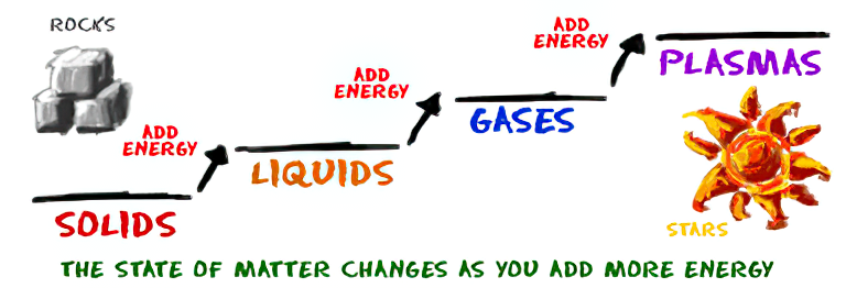
As Einstein showed us, light and matter and just aspects of the same thing. Matter is just frozen light. And light is matter on the move. Albert Einstein’s most famous equation says that energy and matter are two sides of the same coin. How does one become the other?
Relativity requires that the faster an object moves, the more mass it appears to have. This means that somehow part of the energy of the car’s motion appears to transform into mass. Hence the origin of Einstein’s equation. How does that happen? We don’t really know. We only know that it does.
Matter is 99.999999999999 percent empty space. Not only do the atom and solid matter consist mainly of empty space, it is the same in outer space
The quantum theory researchers discovered the answer: Not only do particles consist of energy, but so does the space between. This is the so-called zero-point energy. Therefore it is true: Everything consists of energy.
Energy is the basis of material reality. Every type of particle is conceived of as a quantum vibration in a field: Electrons are vibrations in electron fields, protons vibrate in a proton field, and so on. Everything is energy, and everything is connected to everything else through fields.
DISCLAIMER – Links and images on this website may be protected by the respective owners’ copyright. All data submitted by users through this site shall be treated as freely available to share.