


COMPOSITION


DESIGN
-
Mike Wong – AtoMeow – A Blue noise image stippling in Processing
Read more: Mike Wong – AtoMeow – A Blue noise image stippling in Processing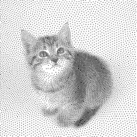
https://github.com/mwkm/atoMeow
https://www.shadertoy.com/view/7s3XzX
This demo is created for coders who are familiar with this awesome creative coding platform. You may quickly modify the code to work for video or to stipple your own Procssing drawings by turning them into
PImageand run the simulation. This demo code also serves as a reference implementation of my article Blue noise sampling using an N-body simulation-based method. If you are interested in 2.5D, you may mod the code to achieve what I discussed in this artist friendly article.Convert your video to a dotted noise.


COLOR
-
FXGuide – ACES 2.0 with ILM’s Alex Fry
Read more: FXGuide – ACES 2.0 with ILM’s Alex Fry
https://draftdocs.acescentral.com/background/whats-new/
ACES 2.0 is the second major release of the components that make up the ACES system. The most significant change is a new suite of rendering transforms whose design was informed by collected feedback and requests from users of ACES 1. The changes aim to improve the appearance of perceived artifacts and to complete previously unfinished components of the system, resulting in a more complete, robust, and consistent product.
Highlights of the key changes in ACES 2.0 are as follows:
- New output transforms, including:
- A less aggressive tone scale
- More intuitive controls to create custom outputs to non-standard displays
- Robust gamut mapping to improve perceptual uniformity
- Improved performance of the inverse transforms
- Enhanced AMF specification
- An updated specification for ACES Transform IDs
- OpenEXR compression recommendations
- Enhanced tools for generating Input Transforms and recommended procedures for characterizing prosumer cameras
- Look Transform Library
- Expanded documentation
Rendering Transform
The most substantial change in ACES 2.0 is a complete redesign of the rendering transform.
ACES 2.0 was built as a unified system, rather than through piecemeal additions. Different deliverable outputs “match” better and making outputs to display setups other than the provided presets is intended to be user-driven. The rendering transforms are less likely to produce undesirable artifacts “out of the box”, which means less time can be spent fixing problematic images and more time making pictures look the way you want.
Key design goals
- Improve consistency of tone scale and provide an easy to use parameter to allow for outputs between preset dynamic ranges
- Minimize hue skews across exposure range in a region of same hue
- Unify for structural consistency across transform type
- Easy to use parameters to create outputs other than the presets
- Robust gamut mapping to improve harsh clipping artifacts
- Fill extents of output code value cube (where appropriate and expected)
- Invertible – not necessarily reversible, but Output > ACES > Output round-trip should be possible
- Accomplish all of the above while maintaining an acceptable “out-of-the box” rendering
- New output transforms, including:
-
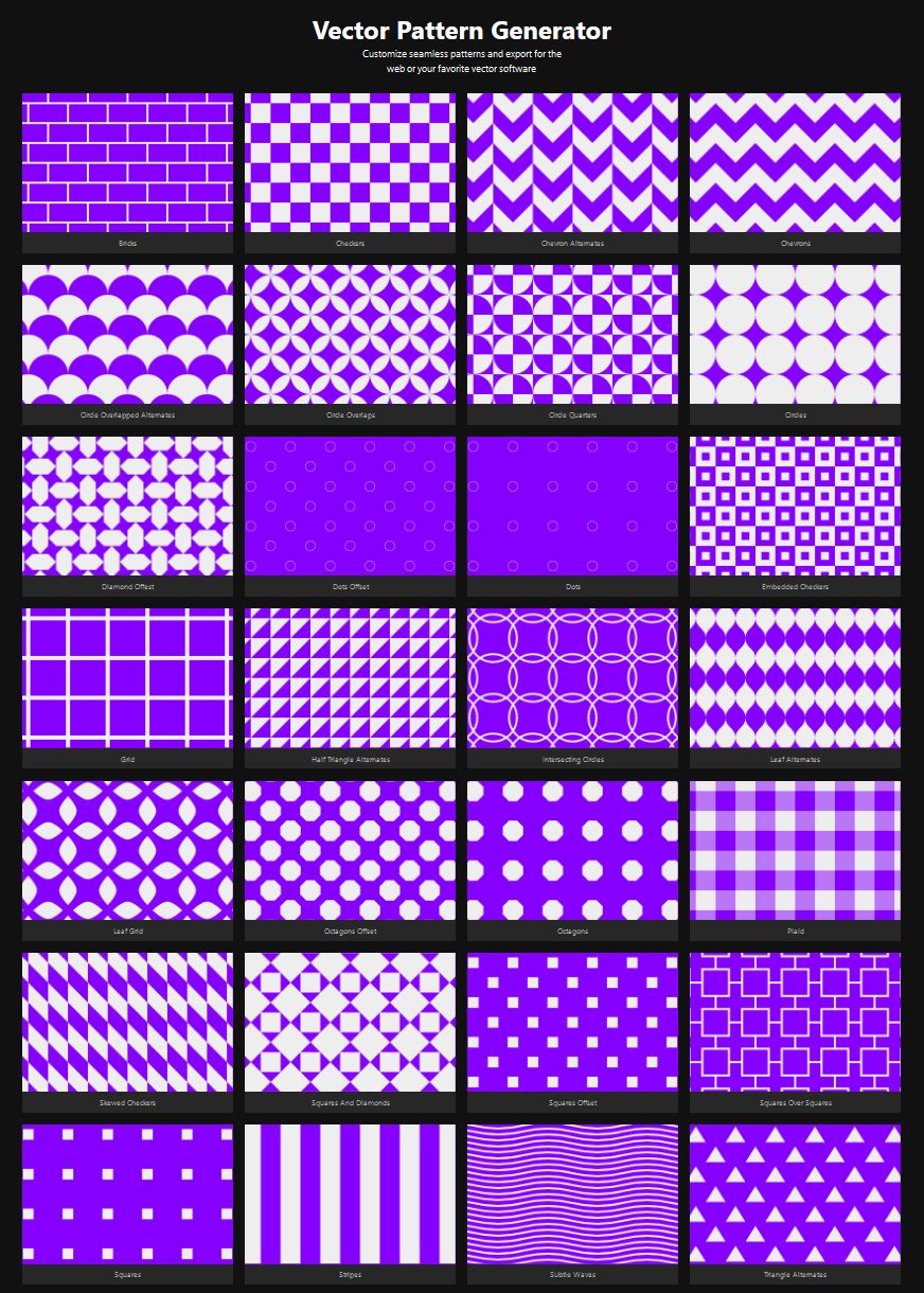
Pattern generators
Read more: Pattern generatorshttp://qrohlf.com/trianglify-generator/
https://halftonepro.com/app/polygons#
https://mattdesl.svbtle.com/generative-art-with-nodejs-and-canvas
https://www.patterncooler.com/
http://permadi.com/java/spaint/spaint.html
https://dribbble.com/shots/1847313-Kaleidoscope-Generator-PSD
http://eskimoblood.github.io/gerstnerizer/
http://www.stripegenerator.com/
http://btmills.github.io/geopattern/geopattern.html
http://fractalarchitect.net/FA4-Random-Generator.html
https://sciencevsmagic.net/fractal/#0605,0000,3,2,0,1,2
https://sites.google.com/site/mandelbulber/home
-
The 7 key elements of brand identity design + 10 corporate identity examples
Read more: The 7 key elements of brand identity design + 10 corporate identity exampleswww.lucidpress.com/blog/the-7-key-elements-of-brand-identity-design
1. Clear brand purpose and positioning
2. Thorough market research
3. Likable brand personality
4. Memorable logo
5. Attractive color palette
6. Professional typography
7. On-brand supporting graphics

-
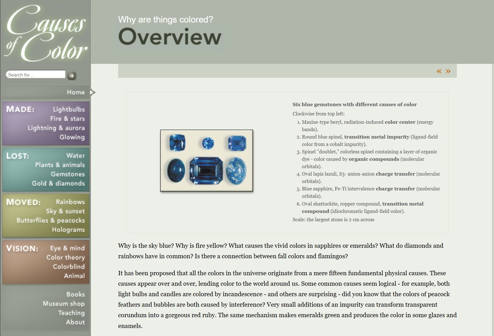
What causes color
Read more: What causes colorwww.webexhibits.org/causesofcolor/5.html
Water itself has an intrinsic blue color that is a result of its molecular structure and its behavior.
-
PTGui 13 beta adds control through a Patch Editor
Read more: PTGui 13 beta adds control through a Patch EditorAdditions:
- Patch Editor (PTGui Pro)
- DNG output
- Improved RAW / DNG handling
- JPEG 2000 support
- Performance improvements

-
sRGB vs REC709 – An introduction and FFmpeg implementations
Read more: sRGB vs REC709 – An introduction and FFmpeg implementations
1. Basic Comparison
- What they are
- sRGB: A standard “web”/computer-display RGB color space defined by IEC 61966-2-1. It’s used for most monitors, cameras, printers, and the vast majority of images on the Internet.
- Rec. 709: An HD-video color space defined by ITU-R BT.709. It’s the go-to standard for HDTV broadcasts, Blu-ray discs, and professional video pipelines.
- Why they exist
- sRGB: Ensures consistent colors across different consumer devices (PCs, phones, webcams).
- Rec. 709: Ensures consistent colors across video production and playback chains (cameras → editing → broadcast → TV).
- What you’ll see
- On your desktop or phone, images tagged sRGB will look “right” without extra tweaking.
- On an HDTV or video-editing timeline, footage tagged Rec. 709 will display accurate contrast and hue on broadcast-grade monitors.
2. Digging Deeper
Feature sRGB Rec. 709 White point D65 (6504 K), same for both D65 (6504 K) Primaries (x,y) R: (0.640, 0.330) G: (0.300, 0.600) B: (0.150, 0.060) R: (0.640, 0.330) G: (0.300, 0.600) B: (0.150, 0.060) Gamut size Identical triangle on CIE 1931 chart Identical to sRGB Gamma / transfer Piecewise curve: approximate 2.2 with linear toe Pure power-law γ≈2.4 (often approximated as 2.2 in practice) Matrix coefficients N/A (pure RGB usage) Y = 0.2126 R + 0.7152 G + 0.0722 B (Rec. 709 matrix) Typical bit-depth 8-bit/channel (with 16-bit variants) 8-bit/channel (10-bit for professional video) Usage metadata Tagged as “sRGB” in image files (PNG, JPEG, etc.) Tagged as “bt709” in video containers (MP4, MOV) Color range Full-range RGB (0–255) Studio-range Y′CbCr (Y′ [16–235], Cb/Cr [16–240])
Why the Small Differences Matter
(more…) - What they are


LIGHTING
-
Photography basics: Lumens vs Candelas (candle) vs Lux vs FootCandle vs Watts vs Irradiance vs Illuminance
Read more: Photography basics: Lumens vs Candelas (candle) vs Lux vs FootCandle vs Watts vs Irradiance vs Illuminancehttps://www.translatorscafe.com/unit-converter/en-US/illumination/1-11/

The power output of a light source is measured using the unit of watts W. This is a direct measure to calculate how much power the light is going to drain from your socket and it is not relatable to the light brightness itself.
The amount of energy emitted from it per second. That energy comes out in a form of photons which we can crudely represent with rays of light coming out of the source. The higher the power the more rays emitted from the source in a unit of time.
Not all energy emitted is visible to the human eye, so we often rely on photometric measurements, which takes in account the sensitivity of human eye to different wavelenghts


Details in the post
(more…) -
Vahan Sosoyan MakeHDR – an OpenFX open source plug-in for merging multiple LDR images into a single HDRI
Read more: Vahan Sosoyan MakeHDR – an OpenFX open source plug-in for merging multiple LDR images into a single HDRIhttps://github.com/Sosoyan/make-hdr
Feature notes
- Merge up to 16 inputs with 8, 10 or 12 bit depth processing
- User friendly logarithmic Tone Mapping controls within the tool
- Advanced controls such as Sampling rate and Smoothness
Available at cross platform on Linux, MacOS and Windows Works consistent in compositing applications like Nuke, Fusion, Natron.
NOTE: The goal is to clean the initial individual brackets before or at merging time as much as possible.
This means:- keeping original shooting metadata
- de-fringing
- removing aberration (through camera lens data or automatically)
- at 32 bit
- in ACEScg (or ACES) wherever possible

-
Custom bokeh in a raytraced DOF render
Read more: Custom bokeh in a raytraced DOF render

To achieve a custom pinhole camera effect with a custom bokeh in Arnold Raytracer, you can follow these steps:
- Set the render camera with a focal length around 50 (or as needed)
- Set the F-Stop to a high value (e.g., 22).
- Set the focus distance as you require
- Turn on DOF
- Place a plane a few cm in front of the camera.
- Texture the plane with a transparent shape at the center of it. (Transmission with no specular roughness)
-
Photography basics: Color Temperature and White Balance
Read more: Photography basics: Color Temperature and White Balance

Color Temperature of a light source describes the spectrum of light which is radiated from a theoretical “blackbody” (an ideal physical body that absorbs all radiation and incident light – neither reflecting it nor allowing it to pass through) with a given surface temperature.
https://en.wikipedia.org/wiki/Color_temperature
Or. Most simply it is a method of describing the color characteristics of light through a numerical value that corresponds to the color emitted by a light source, measured in degrees of Kelvin (K) on a scale from 1,000 to 10,000.
More accurately. The color temperature of a light source is the temperature of an ideal backbody that radiates light of comparable hue to that of the light source.
(more…)


![[gamma correction test]](http://www.madore.org/~david/misc/color/gammatest.png "sRGB gamma correction test")

COLLECTIONS
| Featured AI
| Design And Composition
| Explore posts
POPULAR SEARCHES
unreal | pipeline | virtual production | free | learn | photoshop | 360 | macro | google | nvidia | resolution | open source | hdri | real-time | photography basics | nuke
FEATURED POSTS
-
Canva bought Affinity – Now Affinity Photo and Affinity Designer are… GONE?!
-
Types of Film Lights and their efficiency – CRI, Color Temperature and Luminous Efficacy
-
Blender VideoDepthAI – Turn any video into 3D Animated Scenes
-
QR code logos
-
Steven Stahlberg – Perception and Composition
-
Mastering The Art Of Photography – PixelSham.com Photography Basics
-
Glossary of Lighting Terms – cheat sheet
-
RawTherapee – a free, open source, cross-platform raw image and HDRi processing program
Social Links
DISCLAIMER – Links and images on this website may be protected by the respective owners’ copyright. All data submitted by users through this site shall be treated as freely available to share.
