The intricate relationship between the eyes and the brain, often termed the eye-mind connection, reveals that vision is predominantly a cognitive process. This understanding has profound implications for fields such as design, where capturing and maintaining attention is paramount. This essay delves into the nuances of visual perception, the brain’s role in interpreting visual data, and how this knowledge can be applied to effective design strategies.
This cognitive aspect of vision is evident in phenomena such as optical illusions, where the brain interprets visual information in a way that contradicts physical reality. These illusions underscore that what we “see” is not merely a direct recording of the external world but a constructed experience shaped by cognitive processes.
Understanding the cognitive nature of vision is crucial for effective design. Designers must consider how the brain processes visual information to create compelling and engaging visuals. This involves several key principles:
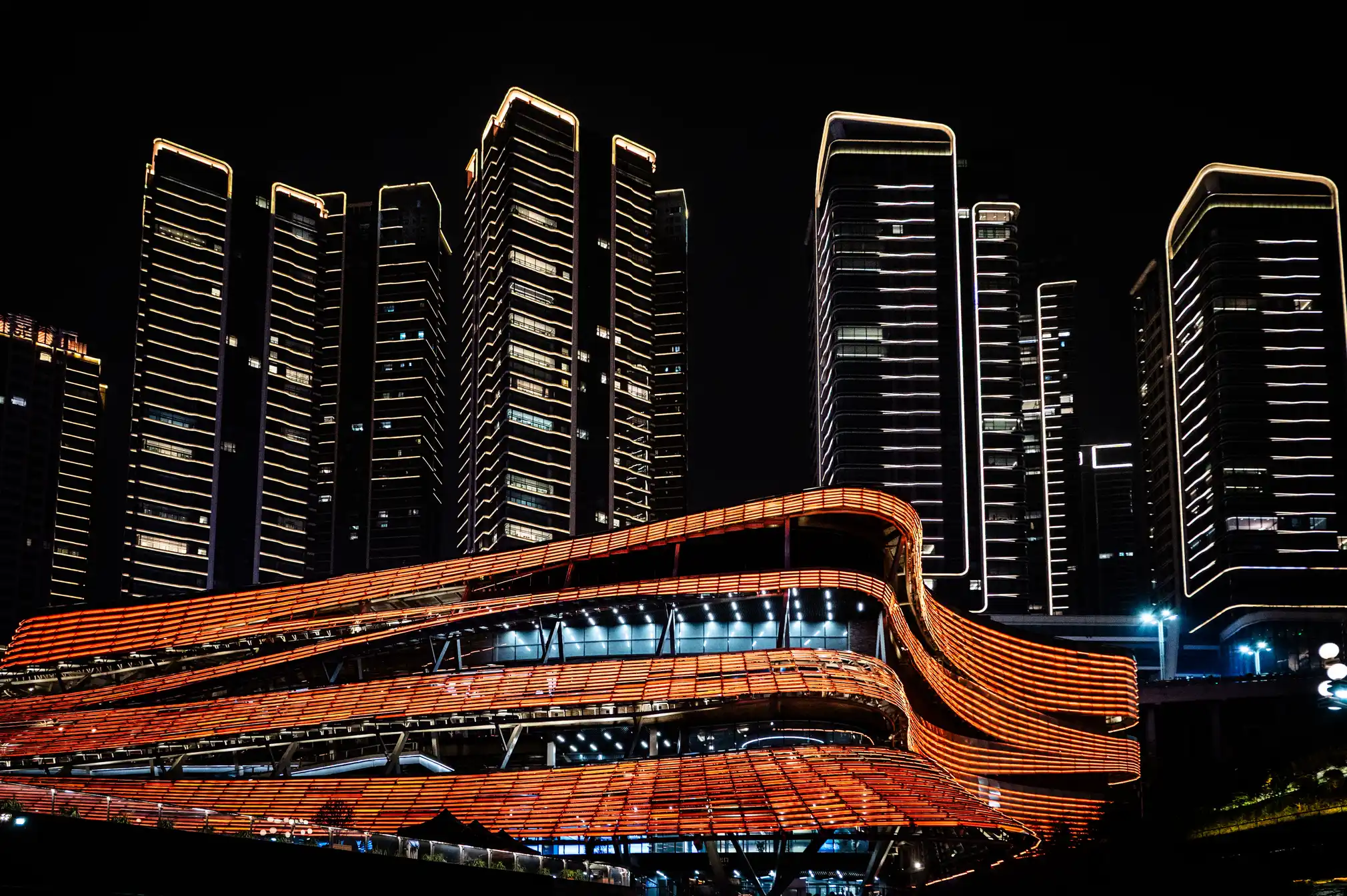
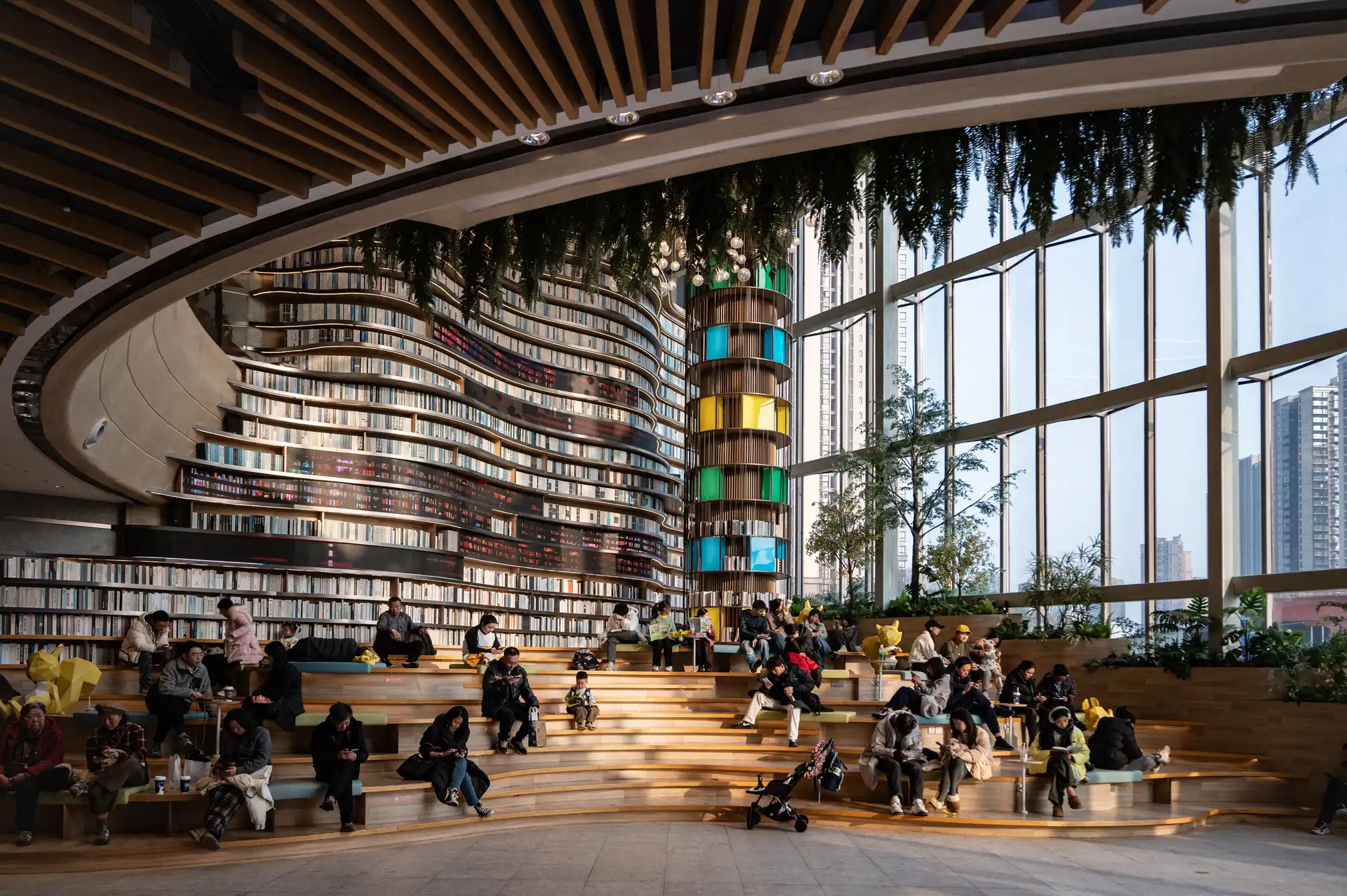
The largest city in the world is as big as Austria, but few people have ever heard of it. The megacity of 34 million people in central of China is the emblem of the fastest urban revolution on the planet.
One problem with sRGB is that in a gradient between blue and white, it becomes a bit purple in the middle of the transition. That’s because sRGB really isn’t created to mimic how the eye sees colors; rather, it is based on how CRT monitors work. That means it works with certain frequencies of red, green, and blue, and also the non-linear coding called gamma. It’s a miracle it works as well as it does, but it’s not connected to color perception. When using those tools, you sometimes get surprising results, like purple in the gradient.
There were also attempts to create simple models matching human perception based on XYZ, but as it turned out, it’s not possible to model all color vision that way. Perception of color is incredibly complex and depends, among other things, on whether it is dark or light in the room and the background color it is against. When you look at a photograph, it also depends on what you think the color of the light source is. The dress is a typical example of color vision being very context-dependent. It is almost impossible to model this perfectly.
I based Oklab on two other color spaces, CIECAM16 and IPT. I used the lightness and saturation prediction from CIECAM16, which is a color appearance model, as a target. I actually wanted to use the datasets used to create CIECAM16, but I couldn’t find them.
IPT was designed to have better hue uniformity. In experiments, they asked people to match light and dark colors, saturated and unsaturated colors, which resulted in a dataset for which colors, subjectively, have the same hue. IPT has a few other issues but is the basis for hue in Oklab.
In the Munsell color system, colors are described with three parameters, designed to match the perceived appearance of colors: Hue, Chroma and Value. The parameters are designed to be independent and each have a uniform scale. This results in a color solid with an irregular shape. The parameters are designed to be independent and each have a uniform scale. This results in a color solid with an irregular shape. Modern color spaces and models, such as CIELAB, Cam16 and Björn Ottosson own Oklab, are very similar in their construction.
By far the most used color spaces today for color picking are HSL and HSV, two representations introduced in the classic 1978 paper “Color Spaces for Computer Graphics”. HSL and HSV designed to roughly correlate with perceptual color properties while being very simple and cheap to compute.
Today HSL and HSV are most commonly used together with the sRGB color space.
One of the main advantages of HSL and HSV over the different Lab color spaces is that they map the sRGB gamut to a cylinder. This makes them easy to use since all parameters can be changed independently, without the risk of creating colors outside of the target gamut.
The main drawback on the other hand is that their properties don’t match human perception particularly well.
Reconciling these conflicting goals perfectly isn’t possible, but given that HSV and HSL don’t use anything derived from experiments relating to human perception, creating something that makes a better tradeoff does not seem unreasonable.
With this new lightness estimate, we are ready to look into the construction of Okhsv and Okhsl.
This paper presents an introduction to the color pipelines behind modern feature-film visual-effects and animation.
Authored by Jeremy Selan, and reviewed by the members of the VES Technology Committee including Rob Bredow, Dan Candela, Nick Cannon, Paul Debevec, Ray Feeney, Andy Hendrickson, Gautham Krishnamurti, Sam Richards, Jordan Soles, and Sebastian Sylwan.
Blind people who regain their sight may find themselves in a world they don’t immediately comprehend. “It would be more like a sighted person trying to rely on tactile information,” Moore says.
Learning to see is a developmental process, just like learning language, Prof Cathleen Moore continues. “As far as vision goes, a three-and-a-half year old child is already a well-calibrated system.”
This help’s us understand the composition of components in/on solar system bodies.
Dips in the observed light spectrum, also known as, lines of absorption occur as gasses absorb energy from light at specific points along the light spectrum.
These dips or darkened zones (lines of absorption) leave a finger print which identify elements and compounds.
In this image the dark absorption bands appear as lines of emission which occur as the result of emitted not reflected (absorbed) light.
In color technology, color depth also known as bit depth, is either the number of bits used to indicate the color of a single pixel, OR the number of bits used for each color component of a single pixel.
When referring to a pixel, the concept can be defined as bits per pixel (bpp).
When referring to a color component, the concept can be defined as bits per component, bits per channel, bits per color (all three abbreviated bpc), and also bits per pixel component, bits per color channel or bits per sample (bps). Modern standards tend to use bits per component, but historical lower-depth systems used bits per pixel more often.
Color depth is only one aspect of color representation, expressing the precision with which the amount of each primary can be expressed; the other aspect is how broad a range of colors can be expressed (the gamut). The definition of both color precision and gamut is accomplished with a color encoding specification which assigns a digital code value to a location in a color space.
import math,sys

def Exposure2Intensity(exposure):
    exp = float(exposure)
    result = math.pow(2,exp)
    print(result)

Exposure2Intensity(0)

def Intensity2Exposure(intensity):
    inarg = float(intensity)

    if inarg == 0:
        print("Exposure of zero intensity is undefined.")
        return

    if inarg < 1e-323:
        inarg = max(inarg, 1e-323)
        print("Exposure of negative intensities is undefined. Clamping to a very small value instead (1e-323)")

    result = math.log(inarg, 2)
    print(result)

Intensity2Exposure(0.1)
Why Exposure?
Exposure is a stop value that multiplies the intensity by 2 to the power of the stop. Increasing exposure by 1 results in double the amount of light.
Artists think in “stops.” Doubling or halving brightness is easy math and common in grading and look-dev. Exposure counts doublings in whole stops:
+1 stop = ×2 brightness
−1 stop = ×0.5 brightness
This gives perceptually even controls across both bright and dark values.
Why Intensity?
Intensity is linear. It’s what render engines and compositors expect when:
Summing values
Averaging pixels
Multiplying or filtering pixel data
Use intensity when you need the actual math on pixel/light data.
Formulas (from your Python)
Intensity from exposure: intensity = 2**exposure
Exposure from intensity: exposure = log₂(intensity)
Guardrails:
Intensity must be > 0 to compute exposure.
If intensity = 0 → exposure is undefined.
Clamp tiny values (e.g. 1e−323) before using log₂.
Use Exposure (stops) when…
You want artist-friendly sliders (−5…+5 stops)
Adjusting look-dev or grading in even stops
Matching plates with quick ±1 stop tweaks
Tweening brightness changes smoothly across ranges
Use Intensity (linear) when…
Storing raw pixel/light values
Multiplying textures or lights by a gain
Performing sums, averages, and filters
Feeding values to render engines expecting linear data
Examples
+2 stops → 2**2 = 4.0 (×4)
+1 stop → 2**1 = 2.0 (×2)
0 stop → 2**0 = 1.0 (×1)
−1 stop → 2**(−1) = 0.5 (×0.5)
−2 stops → 2**(−2) = 0.25 (×0.25)
Intensity 0.1 → exposure = log₂(0.1) ≈ −3.32
Rule of thumb
Think in stops (exposure) for controls and matching. Compute in linear (intensity) for rendering and math.
DISCLAIMER – Links and images on this website may be protected by the respective owners’ copyright. All data submitted by users through this site shall be treated as freely available to share.


 Lines of emission


 Local copy: