


COMPOSITION
-
StudioBinder – Roger Deakins on How to Choose a Camera Lens — Cinematography Composition Techniques
Read more: StudioBinder – Roger Deakins on How to Choose a Camera Lens — Cinematography Composition Techniques
https://www.studiobinder.com/blog/camera-lens-buying-guide/
https://www.studiobinder.com/blog/e-books/camera-lenses-explained-volume-1-ebook


DESIGN
-
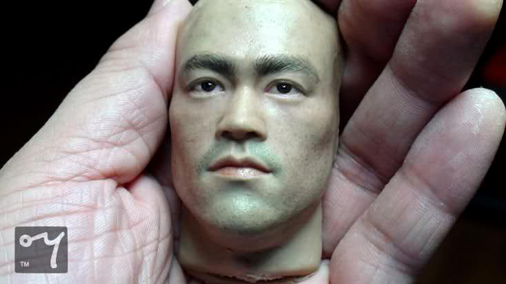
How to paint a boardgame miniatures
Read more: How to paint a boardgame miniatures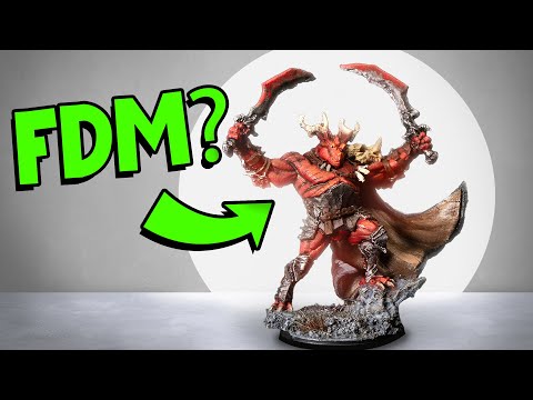
Steps:
- soap wash cleaning
- primer
- base-coat layer (black/white)
- detailing
- washing aka shade (could be done after highlighting)
- highlights aka dry brushing (could be done after washing)
- varnish (gloss/satin/matte)


COLOR
-
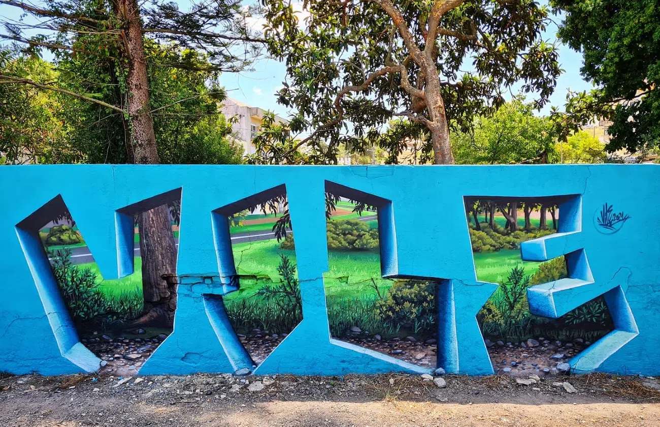
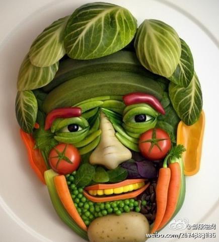
The Maya civilization and the color blue
Read more: The Maya civilization and the color blueMaya blue is a highly unusual pigment because it is a mix of organic indigo and an inorganic clay mineral called palygorskite.
Echoing the color of an azure sky, the indelible pigment was used to accentuate everything from ceramics to human sacrifices in the Late Preclassic period (300 B.C. to A.D. 300).
A team of researchers led by Dean Arnold, an adjunct curator of anthropology at the Field Museum in Chicago, determined that the key to Maya blue was actually a sacred incense called copal.
By heating the mixture of indigo, copal and palygorskite over a fire, the Maya produced the unique pigment, he reported at the time.
-
Stefan Ringelschwandtner – LUT Inspector tool
Read more: Stefan Ringelschwandtner – LUT Inspector toolIt lets you load any .cube LUT right in your browser, see the RGB curves, and use a split view on the Granger Test Image to compare the original vs. LUT-applied version in real time — perfect for spotting hue shifts, saturation changes, and contrast tweaks.
https://mononodes.com/lut-inspector/


-
Photography basics: Lumens vs Candelas (candle) vs Lux vs FootCandle vs Watts vs Irradiance vs Illuminance
Read more: Photography basics: Lumens vs Candelas (candle) vs Lux vs FootCandle vs Watts vs Irradiance vs Illuminancehttps://www.translatorscafe.com/unit-converter/en-US/illumination/1-11/

The power output of a light source is measured using the unit of watts W. This is a direct measure to calculate how much power the light is going to drain from your socket and it is not relatable to the light brightness itself.
The amount of energy emitted from it per second. That energy comes out in a form of photons which we can crudely represent with rays of light coming out of the source. The higher the power the more rays emitted from the source in a unit of time.
Not all energy emitted is visible to the human eye, so we often rely on photometric measurements, which takes in account the sensitivity of human eye to different wavelenghts


Details in the post
(more…) -
Capturing textures albedo
Read more: Capturing textures albedoBuilding a Portable PBR Texture Scanner by Stephane Lb
http://rtgfx.com/pbr-texture-scanner/

How To Split Specular And Diffuse In Real Images, by John Hable
http://filmicworlds.com/blog/how-to-split-specular-and-diffuse-in-real-images/Capturing albedo using a Spectralon
https://www.activision.com/cdn/research/Real_World_Measurements_for_Call_of_Duty_Advanced_Warfare.pdfReal_World_Measurements_for_Call_of_Duty_Advanced_Warfare.pdf
Spectralon is a teflon-based pressed powderthat comes closest to being a pure Lambertian diffuse material that reflects 100% of all light. If we take an HDR photograph of the Spectralon alongside the material to be measured, we can derive thediffuse albedo of that material.

The process to capture diffuse reflectance is very similar to the one outlined by Hable.
1. We put a linear polarizing filter in front of the camera lens and a second linear polarizing filterin front of a modeling light or a flash such that the two filters are oriented perpendicular to eachother, i.e. cross polarized.
2. We place Spectralon close to and parallel with the material we are capturing and take brack-eted shots of the setup7. Typically, we’ll take nine photographs, from -4EV to +4EV in 1EVincrements.
3. We convert the bracketed shots to a linear HDR image. We found that many HDR packagesdo not produce an HDR image in which the pixel values are linear. PTGui is an example of apackage which does generate a linear HDR image. At this point, because of the cross polarization,the image is one of surface diffuse response.
4. We open the file in Photoshop and normalize the image by color picking the Spectralon, filling anew layer with that color and setting that layer to “Divide”. This sets the Spectralon to 1 in theimage. All other color values are relative to this so we can consider them as diffuse albedo.
-
Virtual Production volumes study
Read more: Virtual Production volumes studyColor Fidelity in LED Volumes
https://theasc.com/articles/color-fidelity-in-led-volumes
Virtual Production Glossary
https://vpglossary.com/What is Virtual Production – In depth analysis
https://www.leadingledtech.com/what-is-a-led-virtual-production-studio-in-depth-technical-analysis/
A comparison of LED panels for use in Virtual Production:
Findings and recommendations
https://eprints.bournemouth.ac.uk/36826/1/LED_Comparison_White_Paper%281%29.pdf


LIGHTING
-
Photography basics: Color Temperature and White Balance
Read more: Photography basics: Color Temperature and White Balance

Color Temperature of a light source describes the spectrum of light which is radiated from a theoretical “blackbody” (an ideal physical body that absorbs all radiation and incident light – neither reflecting it nor allowing it to pass through) with a given surface temperature.
https://en.wikipedia.org/wiki/Color_temperature
Or. Most simply it is a method of describing the color characteristics of light through a numerical value that corresponds to the color emitted by a light source, measured in degrees of Kelvin (K) on a scale from 1,000 to 10,000.
More accurately. The color temperature of a light source is the temperature of an ideal backbody that radiates light of comparable hue to that of the light source.
(more…) -
Fast, optimized ‘for’ pixel loops with OpenCV and Python to create tone mapped HDR images
Read more: Fast, optimized ‘for’ pixel loops with OpenCV and Python to create tone mapped HDR imageshttps://pyimagesearch.com/2017/08/28/fast-optimized-for-pixel-loops-with-opencv-and-python/
https://learnopencv.com/exposure-fusion-using-opencv-cpp-python/
Exposure Fusion is a method for combining images taken with different exposure settings into one image that looks like a tone mapped High Dynamic Range (HDR) image.

-
Simulon – a Hollywood production studio app in the hands of an independent creator with access to consumer hardware, LDRi to HDRi through ML
Read more: Simulon – a Hollywood production studio app in the hands of an independent creator with access to consumer hardware, LDRi to HDRi through MLDivesh Naidoo: The video below was made with a live in-camera preview and auto-exposure matching, no camera solve, no HDRI capture and no manual compositing setup. Using the new Simulon phone app.
LDR to HDR through ML
https://simulon.typeform.com/betatest
(more…)Process example


COLLECTIONS
| Featured AI
| Design And Composition
| Explore posts
POPULAR SEARCHES
unreal | pipeline | virtual production | free | learn | photoshop | 360 | macro | google | nvidia | resolution | open source | hdri | real-time | photography basics | nuke
FEATURED POSTS
-
Photography basics: Color Temperature and White Balance
-
Guide to Prompt Engineering
-
Photography basics: Exposure Value vs Photographic Exposure vs Il/Luminance vs Pixel luminance measurements
-
Web vs Printing or digital RGB vs CMYK
-
59 AI Filmmaking Tools For Your Workflow
-
STOP FCC – SAVE THE FREE NET
-
Photography basics: How Exposure Stops (Aperture, Shutter Speed, and ISO) Affect Your Photos – cheat sheet cards
-
Scene Referred vs Display Referred color workflows
Social Links
DISCLAIMER – Links and images on this website may be protected by the respective owners’ copyright. All data submitted by users through this site shall be treated as freely available to share.
