


COMPOSITION
DESIGN
-
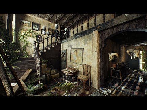
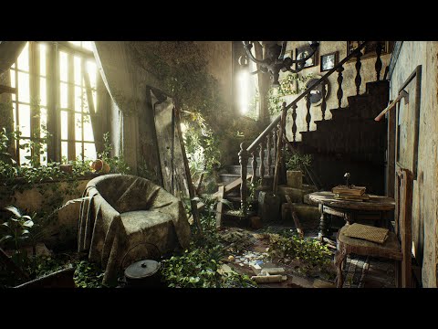
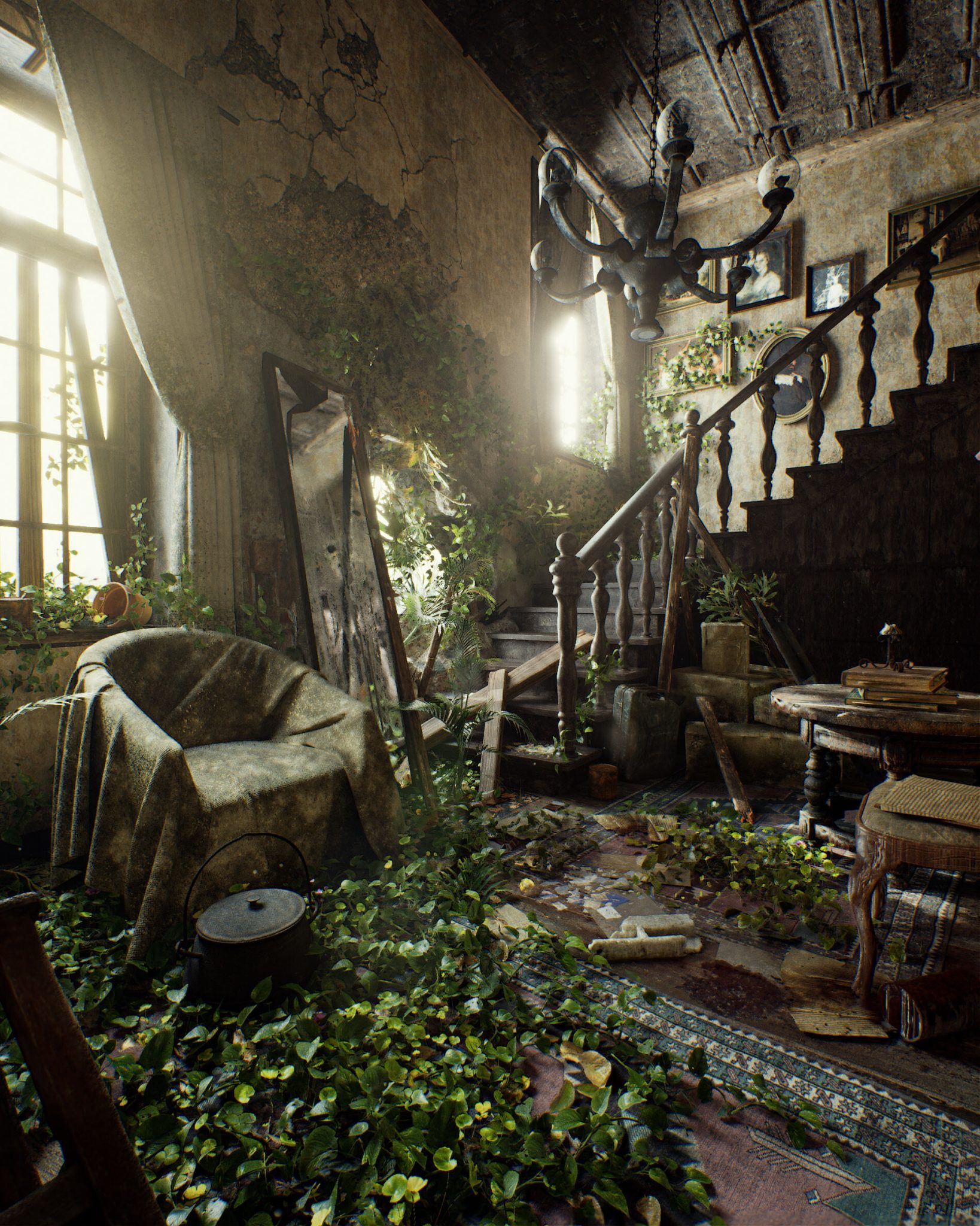
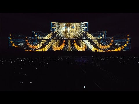
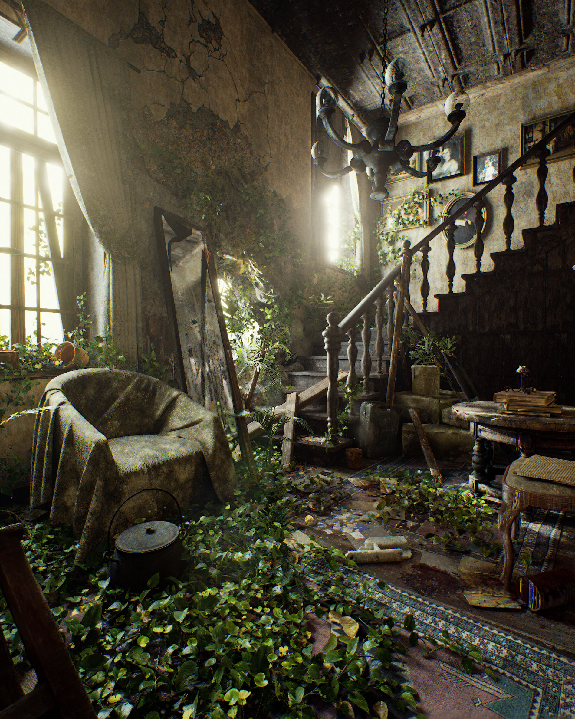
Pasquale Scionti – Production Walkthrough with Virtual Camera and iPad pro 11.5 on Unreal Engine 4.25
Read more: Pasquale Scionti – Production Walkthrough with Virtual Camera and iPad pro 11.5 on Unreal Engine 4.2580.lv/articles/creating-an-old-abandoned-mansion-with-quixel-tools/
www.artstation.com/artwork/Poexyo


COLOR
-
SecretWeapons MixBox – a practical library for paint-like digital color mixing
Read more: SecretWeapons MixBox – a practical library for paint-like digital color mixingInternally, Mixbox treats colors as real-life pigments using the Kubelka & Munk theory to predict realistic color behavior.
https://scrtwpns.com/mixbox/painter/
https://scrtwpns.com/mixbox.pdf
https://github.com/scrtwpns/mixbox
https://scrtwpns.com/mixbox/docs/

-
Is it possible to get a dark yellow
Read more: Is it possible to get a dark yellowhttps://www.patreon.com/posts/102660674
https://www.linkedin.com/posts/stephenwestland_here-is-a-post-about-the-dark-yellow-problem-activity-7187131643764092929-7uCL


LIGHTING
-
Neural Microfacet Fields for Inverse Rendering
Read more: Neural Microfacet Fields for Inverse Renderinghttps://half-potato.gitlab.io/posts/nmf/

-
Tracing Spherical harmonics and how Weta used them in production
Read more: Tracing Spherical harmonics and how Weta used them in productionA way to approximate complex lighting in ultra realistic renders.
All SH lighting techniques involve replacing parts of standard lighting equations with spherical functions that have been projected into frequency space using the spherical harmonics as a basis.
http://www.cs.columbia.edu/~cs4162/slides/spherical-harmonic-lighting.pdf
Spherical harmonics as used at Weta Digital
-
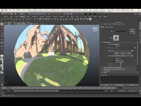
domeble – Hi-Resolution CGI Backplates and 360° HDRI
Read more: domeble – Hi-Resolution CGI Backplates and 360° HDRIWhen collecting hdri make sure the data supports basic metadata, such as:
- Iso
- Aperture
- Exposure time or shutter time
- Color temperature
- Color space Exposure value (what the sensor receives of the sun intensity in lux)
- 7+ brackets (with 5 or 6 being the perceived balanced exposure)
In image processing, computer graphics, and photography, high dynamic range imaging (HDRI or just HDR) is a set of techniques that allow a greater dynamic range of luminances (a Photometry measure of the luminous intensity per unit area of light travelling in a given direction. It describes the amount of light that passes through or is emitted from a particular area, and falls within a given solid angle) between the lightest and darkest areas of an image than standard digital imaging techniques or photographic methods. This wider dynamic range allows HDR images to represent more accurately the wide range of intensity levels found in real scenes ranging from direct sunlight to faint starlight and to the deepest shadows.
The two main sources of HDR imagery are computer renderings and merging of multiple photographs, which in turn are known as low dynamic range (LDR) or standard dynamic range (SDR) images. Tone Mapping (Look-up) techniques, which reduce overall contrast to facilitate display of HDR images on devices with lower dynamic range, can be applied to produce images with preserved or exaggerated local contrast for artistic effect. Photography
In photography, dynamic range is measured in Exposure Values (in photography, exposure value denotes all combinations of camera shutter speed and relative aperture that give the same exposure. The concept was developed in Germany in the 1950s) differences or stops, between the brightest and darkest parts of the image that show detail. An increase of one EV or one stop is a doubling of the amount of light.
The human response to brightness is well approximated by a Steven’s power law, which over a reasonable range is close to logarithmic, as described by the Weber�Fechner law, which is one reason that logarithmic measures of light intensity are often used as well.
HDR is short for High Dynamic Range. It’s a term used to describe an image which contains a greater exposure range than the “black” to “white” that 8 or 16-bit integer formats (JPEG, TIFF, PNG) can describe. Whereas these Low Dynamic Range images (LDR) can hold perhaps 8 to 10 f-stops of image information, HDR images can describe beyond 30 stops and stored in 32 bit images.


COLLECTIONS
| Featured AI
| Design And Composition
| Explore posts
POPULAR SEARCHES
unreal | pipeline | virtual production | free | learn | photoshop | 360 | macro | google | nvidia | resolution | open source | hdri | real-time | photography basics | nuke
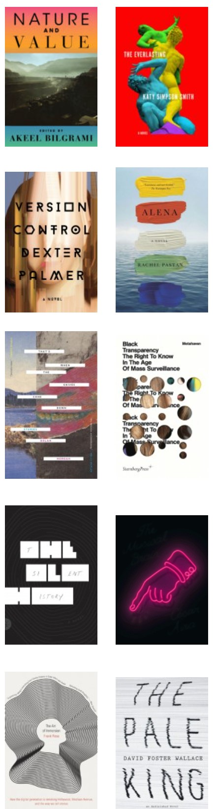
FEATURED POSTS
Social Links
DISCLAIMER – Links and images on this website may be protected by the respective owners’ copyright. All data submitted by users through this site shall be treated as freely available to share.
