this is the epic story of a group of talented digital artists trying to overcame daily technical challenges to achieve incredibly photorealistic projects of monsters and aliens
slowmoVideo is an OpenSource program that creates slow-motion videos from your footage.
Slow motion cinematography is the result of playing back frames for a longer duration than they were exposed. For example, if you expose 240 frames of film in one second, then play them back at 24 fps, the resulting movie is 10 times longer (slower) than the original filmed event….
Film cameras are relatively simple mechanical devices that allow you to crank up the speed to whatever rate the shutter and pull-down mechanism allow. Some film cameras can operate at 2,500 fps or higher (although film shot in these cameras often needs some readjustment in postproduction). Video, on the other hand, is always captured, recorded, and played back at a fixed rate, with a current limit around 60fps. This makes extreme slow motion effects harder to achieve (and less elegant) on video, because slowing down the video results in each frame held still on the screen for a long time, whereas with high-frame-rate film there are plenty of frames to fill the longer durations of time. On video, the slow motion effect is more like a slide show than smooth, continuous motion.
One obvious solution is to shoot film at high speed, then transfer it to video (a case where film still has a clear advantage, sorry George). Another possibility is to cross dissolve or blur from one frame to the next. This adds a smooth transition from one still frame to the next. The blur reduces the sharpness of the image, and compared to slowing down images shot at a high frame rate, this is somewhat of a cheat. However, there isn’t much you can do about it until video can be recorded at much higher rates. Of course, many film cameras can’t shoot at high frame rates either, so the whole super-slow-motion endeavor is somewhat specialized no matter what medium you are using. (There are some high speed digital cameras available now that allow you to capture lots of digital frames directly to your computer, so technology is starting to catch up with film. However, this feature isn’t going to appear in consumer camcorders any time soon.)
To measure the contrast ratio you will need a light meter. The process starts with you measuring the main source of light, or the key light.
Get a reading from the brightest area on the face of your subject. Then, measure the area lit by the secondary light, or fill light. To make sense of what you have just measured you have to understand that the information you have just gathered is in F-stops, a measure of light. With each additional F-stop, for example going one stop from f/1.4 to f/2.0, you create a doubling of light. The reverse is also true; moving one stop from f/8.0 to f/5.6 results in a halving of the light.
A light wave that is vibrating in more than one plane is referred to as unpolarized light. …
Polarized light waves are light waves in which the vibrations occur in a single plane. The process of transforming unpolarized light into polarized light is known as polarization.
The most common use of polarized technology is to reduce lighting complexity on the subject. Details such as glare and hard edges are not removed, but greatly reduced.
While the human eye has red, green, and blue-sensing cones, those cones are cross-wired in the retina to produce a luminance channel plus a red-green and a blue-yellow channel, and it’s data in that color space (known technically as “LAB”) that goes to the brain. That’s why we can’t perceive a reddish-green or a yellowish-blue, whereas such colors can be represented in the RGB color space used by digital cameras.
The back of the retina is covered in light-sensitive neurons known as cone cells and rod cells. There are three types of cone cells, each sensitive to different ranges of light. These ranges overlap, but for convenience the cones are referred to as blue (short-wavelength), green (medium-wavelength), and red (long-wavelength). The rod cells are primarily used in low-light situations, so we’ll ignore those for now.
When light enters the eye and hits the cone cells, the cones get excited and send signals to the brain through the visual cortex. Different wavelengths of light excite different combinations of cones to varying levels, which generates our perception of color. You can see that the red cones are most sensitive to light, and the blue cones are least sensitive. The sensitivity of green and red cones overlaps for most of the visible spectrum.
Here’s how your brain takes the signals of light intensity from the cones and turns it into color information. To see red or green, your brain finds the difference between the levels of excitement in your red and green cones. This is the red-green channel.
To get “brightness,” your brain combines the excitement of your red and green cones. This creates the luminance, or black-white, channel. To see yellow or blue, your brain then finds the difference between this luminance signal and the excitement of your blue cones. This is the yellow-blue channel.
From the calculations made in the brain along those three channels, we get four basic colors: blue, green, yellow, and red. Seeing blue is what you experience when low-wavelength light excites the blue cones more than the green and red.
Seeing green happens when light excites the green cones more than the red cones. Seeing red happens when only the red cones are excited by high-wavelength light.
Here’s where it gets interesting. Seeing yellow is what happens when BOTH the green AND red cones are highly excited near their peak sensitivity. This is the biggest collective excitement that your cones ever have, aside from seeing pure white.
Notice that yellow occurs at peak intensity in the graph to the right. Further, the lens and cornea of the eye happen to block shorter wavelengths, reducing sensitivity to blue and violet light.
A LUT (Lookup Table) is essentially the modifier between two images, the original image and the displayed image, based on a mathematical formula. Basically conversion matrices of different complexities. There are different types of LUTS – viewing, transform, calibration, 1D and 3D.
The dynamic range is a ratio between the maximum and minimum values of a physical measurement. Its definition depends on what the dynamic range refers to.
For a scene: Dynamic range is the ratio between the brightest and darkest parts of the scene.
For a camera: Dynamic range is the ratio of saturation to noise. More specifically, the ratio of the intensity that just saturates the camera to the intensity that just lifts the camera response one standard deviation above camera noise.
For a display: Dynamic range is the ratio between the maximum and minimum intensities emitted from the screen.
The Dynamic Range of real-world scenes can be quite high — ratios of 100,000:1 are common in the natural world. An HDR (High Dynamic Range) image stores pixel values that span the whole tonal range of real-world scenes. Therefore, an HDR image is encoded in a format that allows the largest range of values, e.g. floating-point values stored with 32 bits per color channel. Another characteristics of an HDR image is that it stores linear values. This means that the value of a pixel from an HDR image is proportional to the amount of light measured by the camera.
For TVs HDR is great, but it’s not the only new TV feature worth discussing.
Note: In Foundry’s Nuke, the software will map 18% gray to whatever your center f/stop is set to in the viewer settings (f/8 by default… change that to EV by following the instructions below).
You can experiment with this by attaching an Exposure node to a Constant set to 0.18, setting your viewer read-out to Spotmeter, and adjusting the stops in the node up and down. You will see that a full stop up or down will give you the respective next value on the aperture scale (f8, f11, f16 etc.).
One stop doubles or halves the amount or light that hits the filmback/ccd, so everything works in powers of 2.
So starting with 0.18 in your constant, you will see that raising it by a stop will give you .36 as a floating point number (in linear space), while your f/stop will be f/11 and so on.
If you set your center stop to 0 (see below) you will get a relative readout in EVs, where EV 0 again equals 18% constant gray.
In other words. Setting the center f-stop to 0 means that in a neutral plate, the middle gray in the macbeth chart will equal to exposure value 0. EV 0 corresponds to an exposure time of 1 sec and an aperture of f/1.0.
This will set the sun usually around EV12-17 and the sky EV1-4 , depending on cloud coverage.
To switch Foundry’s Nuke’s SpotMeter to return the EV of an image, click on the main viewport, and then press s, this opens the viewer’s properties. Now set the center f-stop to 0 in there. And the SpotMeter in the viewport will change from aperture and fstops to EV.
“Fix your gaze on the black dot on the left side of this image. But wait! Finish reading this paragraph first. As you gaze at the left dot, try to answer this question: In what direction is the object on the right moving? Is it drifting diagonally, or is it moving up and down?”
Answering the question that is often asked, “Do I need to use ACEScg to display an sRGB monitor in the end?” (Demonstration shown at an in-house seminar) Comparison of scanlineRender output with extreme color lights on color charts with sRGB/ACREScg in color – OCIO -working space in Nuke
One problem with sRGB is that in a gradient between blue and white, it becomes a bit purple in the middle of the transition. That’s because sRGB really isn’t created to mimic how the eye sees colors; rather, it is based on how CRT monitors work. That means it works with certain frequencies of red, green, and blue, and also the non-linear coding called gamma. It’s a miracle it works as well as it does, but it’s not connected to color perception. When using those tools, you sometimes get surprising results, like purple in the gradient.
There were also attempts to create simple models matching human perception based on XYZ, but as it turned out, it’s not possible to model all color vision that way. Perception of color is incredibly complex and depends, among other things, on whether it is dark or light in the room and the background color it is against. When you look at a photograph, it also depends on what you think the color of the light source is. The dress is a typical example of color vision being very context-dependent. It is almost impossible to model this perfectly.
I based Oklab on two other color spaces, CIECAM16 and IPT. I used the lightness and saturation prediction from CIECAM16, which is a color appearance model, as a target. I actually wanted to use the datasets used to create CIECAM16, but I couldn’t find them.
IPT was designed to have better hue uniformity. In experiments, they asked people to match light and dark colors, saturated and unsaturated colors, which resulted in a dataset for which colors, subjectively, have the same hue. IPT has a few other issues but is the basis for hue in Oklab.
In the Munsell color system, colors are described with three parameters, designed to match the perceived appearance of colors: Hue, Chroma and Value. The parameters are designed to be independent and each have a uniform scale. This results in a color solid with an irregular shape. The parameters are designed to be independent and each have a uniform scale. This results in a color solid with an irregular shape. Modern color spaces and models, such as CIELAB, Cam16 and Björn Ottosson own Oklab, are very similar in their construction.
By far the most used color spaces today for color picking are HSL and HSV, two representations introduced in the classic 1978 paper “Color Spaces for Computer Graphics”. HSL and HSV designed to roughly correlate with perceptual color properties while being very simple and cheap to compute.
Today HSL and HSV are most commonly used together with the sRGB color space.
One of the main advantages of HSL and HSV over the different Lab color spaces is that they map the sRGB gamut to a cylinder. This makes them easy to use since all parameters can be changed independently, without the risk of creating colors outside of the target gamut.
The main drawback on the other hand is that their properties don’t match human perception particularly well.
Reconciling these conflicting goals perfectly isn’t possible, but given that HSV and HSL don’t use anything derived from experiments relating to human perception, creating something that makes a better tradeoff does not seem unreasonable.
With this new lightness estimate, we are ready to look into the construction of Okhsv and Okhsl.
Artificial light sources, not unlike the diverse phases of natural light, vary considerably in their properties. As a result, some lamps render an object’s color better than others do.
The most important criterion for assessing the color-rendering ability of any lamp is its spectral power distribution curve.
Natural daylight varies too much in strength and spectral composition to be taken seriously as a lighting standard for grading and dealing colored stones. For anything to be a standard, it must be constant in its properties, which natural light is not.
For dealers in particular to make the transition from natural light to an artificial light source, that source must offer:
1- A degree of illuminance at least as strong as the common phases of natural daylight.
2- Spectral properties identical or comparable to a phase of natural daylight.
A source combining these two things makes gems appear much the same as when viewed under a given phase of natural light. From the viewpoint of many dealers, this corresponds to a naturalappearance.
The 6000° Kelvin xenon short-arc lamp appears closest to meeting the criteria for a standard light source. Besides the strong illuminance this lamp affords, its spectrum is very similar to CIE standard illuminants of similar color temperature.
A way to approximate complex lighting in ultra realistic renders.
All SH lighting techniques involve replacing parts of standard lighting equations with spherical functions that have been projected into frequency space using the spherical harmonics as a basis.
DISCLAIMER – Links and images on this website may be protected by the respective owners’ copyright. All data submitted by users through this site shall be treated as freely available to share.