


COMPOSITION
-
StudioBinder – Roger Deakins on How to Choose a Camera Lens — Cinematography Composition Techniques
Read more: StudioBinder – Roger Deakins on How to Choose a Camera Lens — Cinematography Composition Techniques
https://www.studiobinder.com/blog/camera-lens-buying-guide/
https://www.studiobinder.com/blog/e-books/camera-lenses-explained-volume-1-ebook
-
Photography basics: Depth of Field and composition
Read more: Photography basics: Depth of Field and compositionDepth of field is the range within which focusing is resolved in a photo.
Aperture has a huge affect on to the depth of field.
Changing the f-stops (f/#) of a lens will change aperture and as such the DOF.
f-stops are a just certain number which is telling you the size of the aperture. That’s how f-stop is related to aperture (and DOF).
If you increase f-stops, it will increase DOF, the area in focus (and decrease the aperture). On the other hand, decreasing the f-stop it will decrease DOF (and increase the aperture).
The red cone in the figure is an angular representation of the resolution of the system. Versus the dotted lines, which indicate the aperture coverage. Where the lines of the two cones intersect defines the total range of the depth of field.
This image explains why the longer the depth of field, the greater the range of clarity.


DESIGN
-
boldtron – 𝗗𝗘𝗣𝗜𝗖𝗧𝗜𝗡𝗚 𝗪𝗔𝗧𝗘𝗥𝗚𝗨𝗡𝗦
Read more: boldtron – 𝗗𝗘𝗣𝗜𝗖𝗧𝗜𝗡𝗚 𝗪𝗔𝗧𝗘𝗥𝗚𝗨𝗡𝗦See this Instagram post by @boldtron using ComfyUI + Krea
https://www.instagram.com/p/C5v-H0PNYYg/?utm_source=ig_web_button_share_sheet


COLOR
-
Akiyoshi Kitaoka – Surround biased illumination perception
Read more: Akiyoshi Kitaoka – Surround biased illumination perceptionhttps://x.com/AkiyoshiKitaoka/status/1798705648001327209
The left face appears whitish and the right one blackish, but they are made up of the same luminance.

https://community.wolfram.com/groups/-/m/t/3191015
Illusory staircase Gelb effect
https://www.psy.ritsumei.ac.jp/akitaoka/illgelbe.html
-
colorhunt.co
Read more: colorhunt.coColor Hunt is a free and open platform for color inspiration with thousands of trendy hand-picked color palettes.

-
What Is The Resolution and view coverage Of The human Eye. And what distance is TV at best?
Read more: What Is The Resolution and view coverage Of The human Eye. And what distance is TV at best?
https://www.discovery.com/science/mexapixels-in-human-eye
About 576 megapixels for the entire field of view.
Consider a view in front of you that is 90 degrees by 90 degrees, like looking through an open window at a scene. The number of pixels would be:
90 degrees * 60 arc-minutes/degree * 1/0.3 * 90 * 60 * 1/0.3 = 324,000,000 pixels (324 megapixels).At any one moment, you actually do not perceive that many pixels, but your eye moves around the scene to see all the detail you want. But the human eye really sees a larger field of view, close to 180 degrees. Let’s be conservative and use 120 degrees for the field of view. Then we would see:
120 * 120 * 60 * 60 / (0.3 * 0.3) = 576 megapixels.
Or.
7 megapixels for the 2 degree focus arc… + 1 megapixel for the rest.
https://clarkvision.com/articles/eye-resolution.html
Details in the post
-
The Forbidden colors – Red-Green & Blue-Yellow: The Stunning Colors You Can’t See
Read more: The Forbidden colors – Red-Green & Blue-Yellow: The Stunning Colors You Can’t Seewww.livescience.com/17948-red-green-blue-yellow-stunning-colors.html

While the human eye has red, green, and blue-sensing cones, those cones are cross-wired in the retina to produce a luminance channel plus a red-green and a blue-yellow channel, and it’s data in that color space (known technically as “LAB”) that goes to the brain. That’s why we can’t perceive a reddish-green or a yellowish-blue, whereas such colors can be represented in the RGB color space used by digital cameras.
https://en.rockcontent.com/blog/the-use-of-yellow-in-data-design
The back of the retina is covered in light-sensitive neurons known as cone cells and rod cells. There are three types of cone cells, each sensitive to different ranges of light. These ranges overlap, but for convenience the cones are referred to as blue (short-wavelength), green (medium-wavelength), and red (long-wavelength). The rod cells are primarily used in low-light situations, so we’ll ignore those for now.
When light enters the eye and hits the cone cells, the cones get excited and send signals to the brain through the visual cortex. Different wavelengths of light excite different combinations of cones to varying levels, which generates our perception of color. You can see that the red cones are most sensitive to light, and the blue cones are least sensitive. The sensitivity of green and red cones overlaps for most of the visible spectrum.

Here’s how your brain takes the signals of light intensity from the cones and turns it into color information. To see red or green, your brain finds the difference between the levels of excitement in your red and green cones. This is the red-green channel.
To get “brightness,” your brain combines the excitement of your red and green cones. This creates the luminance, or black-white, channel. To see yellow or blue, your brain then finds the difference between this luminance signal and the excitement of your blue cones. This is the yellow-blue channel.
From the calculations made in the brain along those three channels, we get four basic colors: blue, green, yellow, and red. Seeing blue is what you experience when low-wavelength light excites the blue cones more than the green and red.
Seeing green happens when light excites the green cones more than the red cones. Seeing red happens when only the red cones are excited by high-wavelength light.
Here’s where it gets interesting. Seeing yellow is what happens when BOTH the green AND red cones are highly excited near their peak sensitivity. This is the biggest collective excitement that your cones ever have, aside from seeing pure white.
Notice that yellow occurs at peak intensity in the graph to the right. Further, the lens and cornea of the eye happen to block shorter wavelengths, reducing sensitivity to blue and violet light.
-
OpenColorIO standard
Read more: OpenColorIO standardhttps://www.provideocoalition.com/color-management-part-11-introducing-opencolorio/
OpenColorIO (OCIO) is a new open source project from Sony Imageworks.
Based on development started in 2003, OCIO enables color transforms and image display to be handled in a consistent manner across multiple graphics applications. Unlike other color management solutions, OCIO is geared towards motion-picture post production, with an emphasis on visual effects and animation color pipelines.

-
Photography basics: Lumens vs Candelas (candle) vs Lux vs FootCandle vs Watts vs Irradiance vs Illuminance
Read more: Photography basics: Lumens vs Candelas (candle) vs Lux vs FootCandle vs Watts vs Irradiance vs Illuminancehttps://www.translatorscafe.com/unit-converter/en-US/illumination/1-11/

The power output of a light source is measured using the unit of watts W. This is a direct measure to calculate how much power the light is going to drain from your socket and it is not relatable to the light brightness itself.
The amount of energy emitted from it per second. That energy comes out in a form of photons which we can crudely represent with rays of light coming out of the source. The higher the power the more rays emitted from the source in a unit of time.
Not all energy emitted is visible to the human eye, so we often rely on photometric measurements, which takes in account the sensitivity of human eye to different wavelenghts


Details in the post
(more…)


LIGHTING
-
What light is best to illuminate gems for resale
Read more: What light is best to illuminate gems for resalewww.palagems.com/gem-lighting2
Artificial light sources, not unlike the diverse phases of natural light, vary considerably in their properties. As a result, some lamps render an object’s color better than others do.
The most important criterion for assessing the color-rendering ability of any lamp is its spectral power distribution curve.
Natural daylight varies too much in strength and spectral composition to be taken seriously as a lighting standard for grading and dealing colored stones. For anything to be a standard, it must be constant in its properties, which natural light is not.
For dealers in particular to make the transition from natural light to an artificial light source, that source must offer:
1- A degree of illuminance at least as strong as the common phases of natural daylight.
2- Spectral properties identical or comparable to a phase of natural daylight.A source combining these two things makes gems appear much the same as when viewed under a given phase of natural light. From the viewpoint of many dealers, this corresponds to a naturalappearance.
The 6000° Kelvin xenon short-arc lamp appears closest to meeting the criteria for a standard light source. Besides the strong illuminance this lamp affords, its spectrum is very similar to CIE standard illuminants of similar color temperature.


-
Gamma correction
Read more: Gamma correction

http://www.normankoren.com/makingfineprints1A.html#Gammabox
https://en.wikipedia.org/wiki/Gamma_correction
http://www.photoscientia.co.uk/Gamma.htm
https://www.w3.org/Graphics/Color/sRGB.html
http://www.eizoglobal.com/library/basics/lcd_display_gamma/index.html
https://forum.reallusion.com/PrintTopic308094.aspx
Basically, gamma is the relationship between the brightness of a pixel as it appears on the screen, and the numerical value of that pixel. Generally Gamma is just about defining relationships.
Three main types:
– Image Gamma encoded in images
– Display Gammas encoded in hardware and/or viewing time
– System or Viewing Gamma which is the net effect of all gammas when you look back at a final image. In theory this should flatten back to 1.0 gamma.
(more…) -
How to Direct and Edit a Fight Scene for Rhythm and Pacing
Read more: How to Direct and Edit a Fight Scene for Rhythm and Pacingwww.premiumbeat.com/blog/directing-fight-scene-cinematography/

1- Frame the action
2- Stage the action
3- Use camera movements
4- Set a rhythm
5- Control the speed of the action
-
Unity 3D resources
Read more: Unity 3D resources
http://answers.unity3d.com/questions/12321/how-can-i-start-learning-unity-fast-list-of-tutori.html
If you have no previous experience with Unity, start with these six video tutorials which give a quick overview of the Unity interface and some important features http://unity3d.com/support/documentation/video/
-
Composition and The Expressive Nature Of Light
Read more: Composition and The Expressive Nature Of Lighthttp://www.huffingtonpost.com/bill-danskin/post_12457_b_10777222.html
George Sand once said “ The artist vocation is to send light into the human heart.”

-
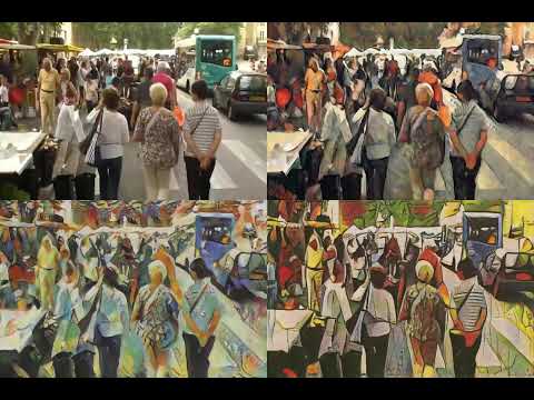
Fast, optimized ‘for’ pixel loops with OpenCV and Python to create tone mapped HDR images
Read more: Fast, optimized ‘for’ pixel loops with OpenCV and Python to create tone mapped HDR imageshttps://pyimagesearch.com/2017/08/28/fast-optimized-for-pixel-loops-with-opencv-and-python/
https://learnopencv.com/exposure-fusion-using-opencv-cpp-python/
Exposure Fusion is a method for combining images taken with different exposure settings into one image that looks like a tone mapped High Dynamic Range (HDR) image.


COLLECTIONS
| Featured AI
| Design And Composition
| Explore posts
POPULAR SEARCHES
unreal | pipeline | virtual production | free | learn | photoshop | 360 | macro | google | nvidia | resolution | open source | hdri | real-time | photography basics | nuke
FEATURED POSTS
-
Principles of Animation with Alan Becker, Dermot OConnor and Shaun Keenan
-
ComfyDock – The Easiest (Free) Way to Safely Run ComfyUI Sessions in a Boxed Container
-
NVidia – High-Fidelity 3D Mesh Generation at Scale with Meshtron
-
ComfyUI FLOAT – A container for FLOAT Generative Motion Latent Flow Matching for Audio-driven Talking Portrait – lip sync
-
Photography basics: Solid Angle measures
-
59 AI Filmmaking Tools For Your Workflow
-
Eddie Yoon – There’s a big misconception about AI creative
-
Scene Referred vs Display Referred color workflows
Social Links
DISCLAIMER – Links and images on this website may be protected by the respective owners’ copyright. All data submitted by users through this site shall be treated as freely available to share.
