


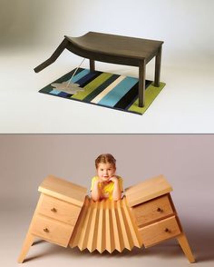
COMPOSITION
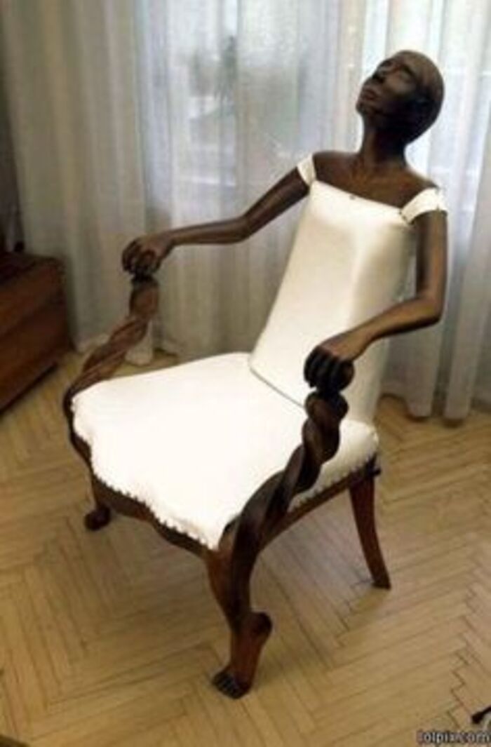
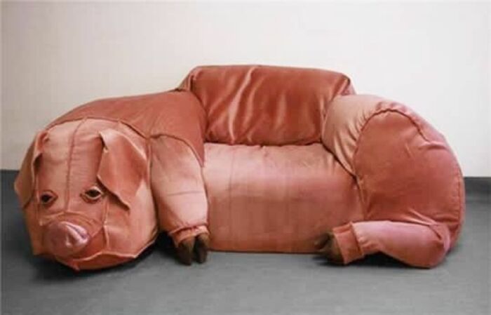
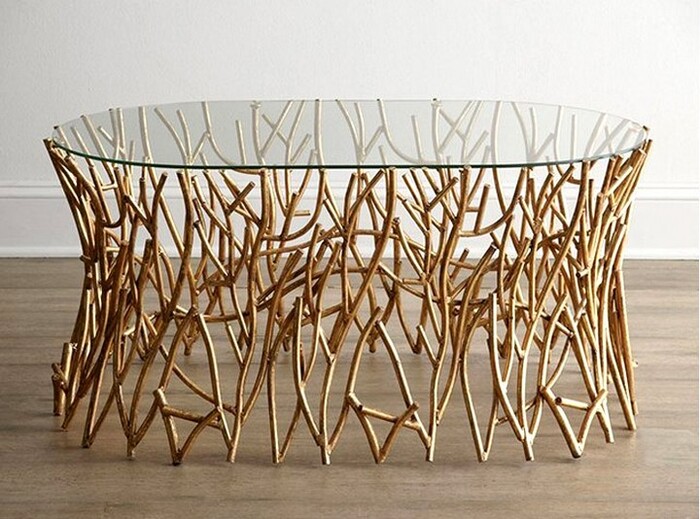
DESIGN


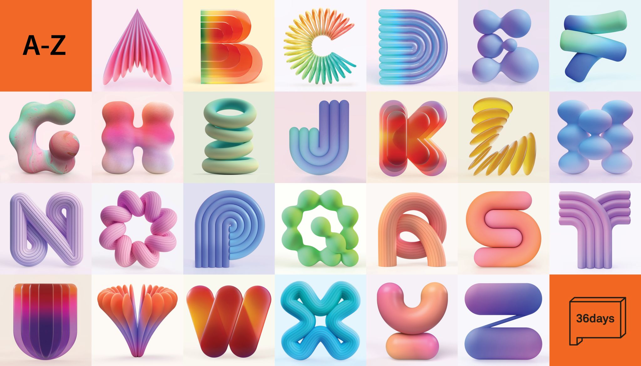
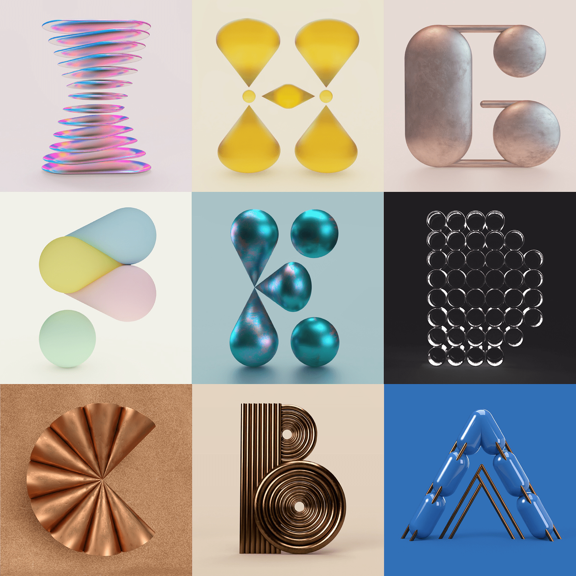
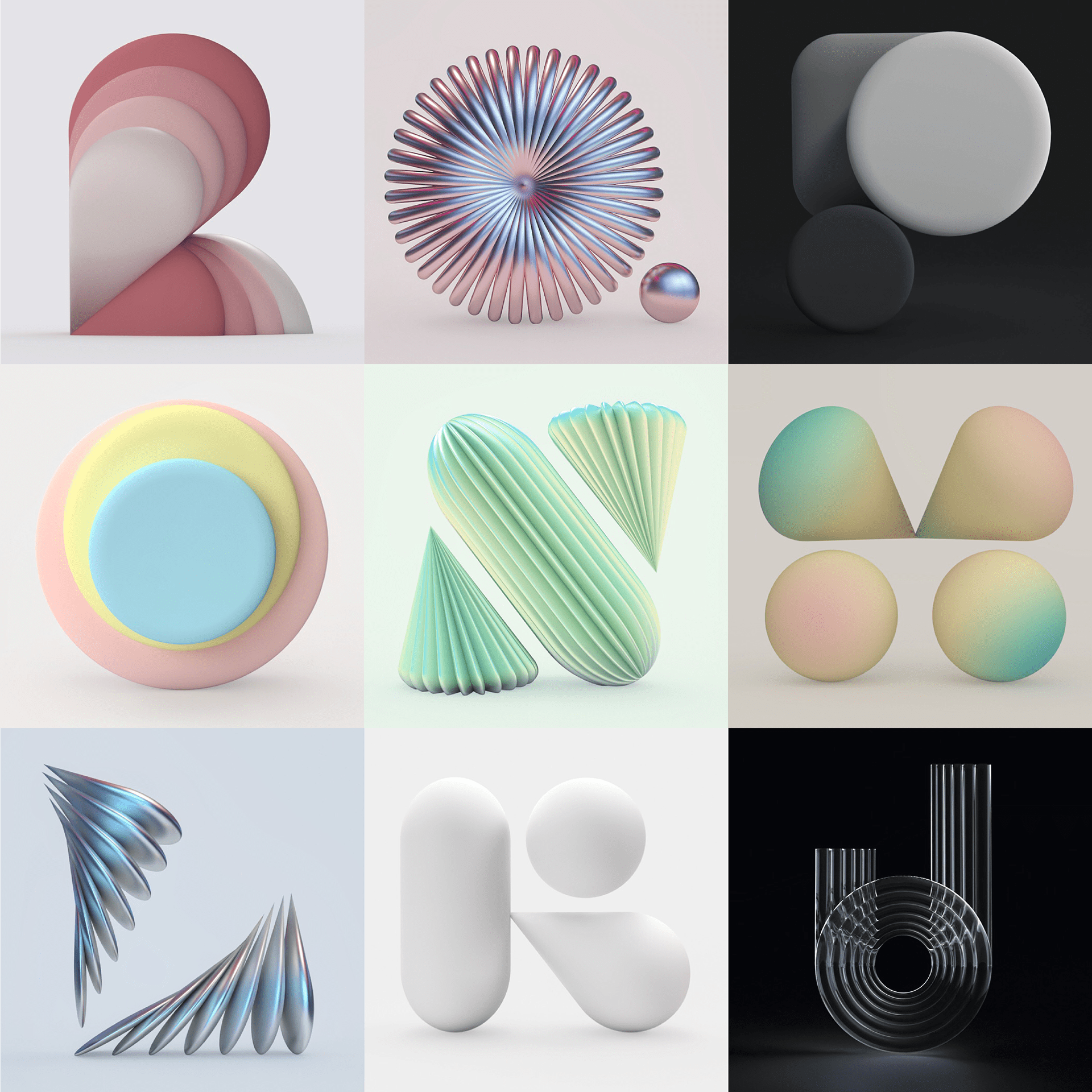

COLOR
-
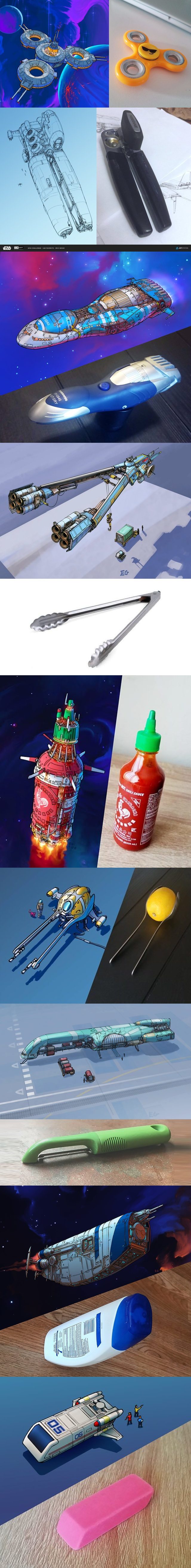
Brett Jones / Phil Reyneri (Lightform) / Philipp7pc: The study of Projection Mapping through Projectors
Read more: Brett Jones / Phil Reyneri (Lightform) / Philipp7pc: The study of Projection Mapping through Projectors


Video Projection Tool Software
https://hcgilje.wordpress.com/vpt/
https://www.projectorpoint.co.uk/news/how-bright-should-my-projector-be/
http://www.adwindowscreens.com/the_calculator/
heavym
https://heavym.net/en/
MadMapper
https://madmapper.com/
-
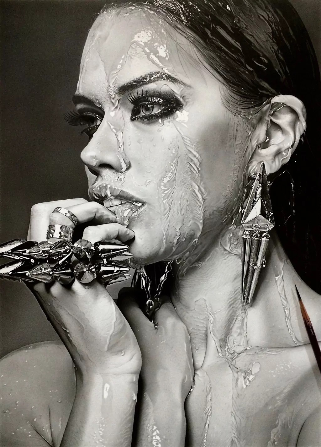
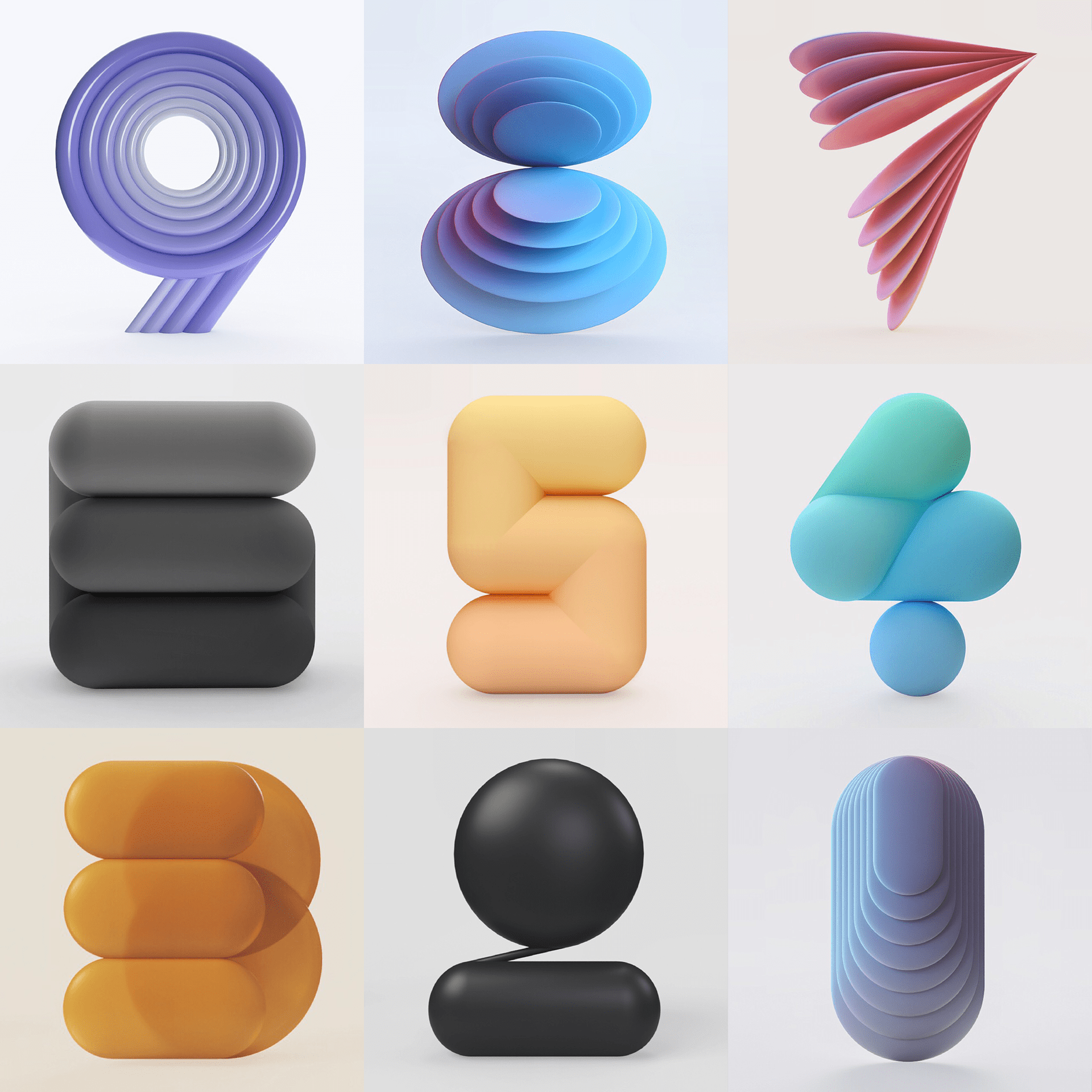
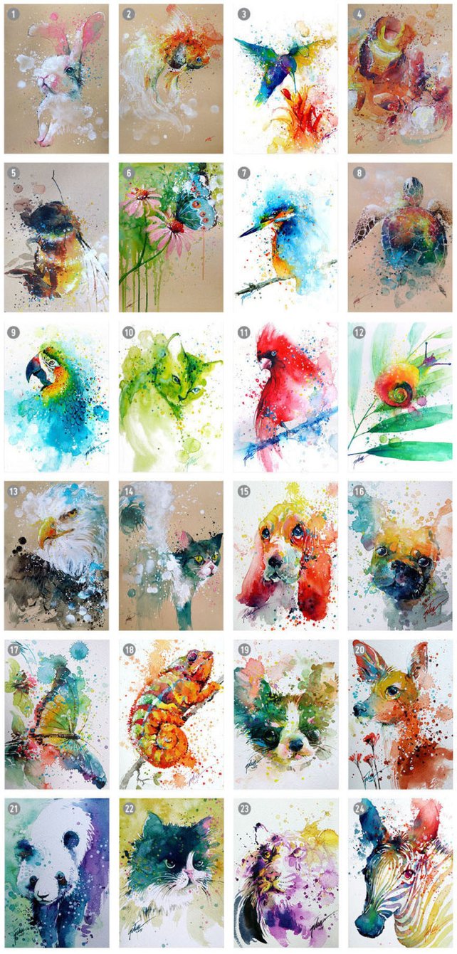
SecretWeapons MixBox – a practical library for paint-like digital color mixing
Read more: SecretWeapons MixBox – a practical library for paint-like digital color mixingInternally, Mixbox treats colors as real-life pigments using the Kubelka & Munk theory to predict realistic color behavior.
https://scrtwpns.com/mixbox/painter/
https://scrtwpns.com/mixbox.pdf
https://github.com/scrtwpns/mixbox
https://scrtwpns.com/mixbox/docs/

-
Photography basics: Lumens vs Candelas (candle) vs Lux vs FootCandle vs Watts vs Irradiance vs Illuminance
Read more: Photography basics: Lumens vs Candelas (candle) vs Lux vs FootCandle vs Watts vs Irradiance vs Illuminancehttps://www.translatorscafe.com/unit-converter/en-US/illumination/1-11/

The power output of a light source is measured using the unit of watts W. This is a direct measure to calculate how much power the light is going to drain from your socket and it is not relatable to the light brightness itself.
The amount of energy emitted from it per second. That energy comes out in a form of photons which we can crudely represent with rays of light coming out of the source. The higher the power the more rays emitted from the source in a unit of time.
Not all energy emitted is visible to the human eye, so we often rely on photometric measurements, which takes in account the sensitivity of human eye to different wavelenghts


Details in the post
(more…) -
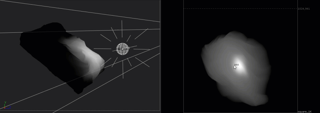
Capturing textures albedo
Read more: Capturing textures albedoBuilding a Portable PBR Texture Scanner by Stephane Lb
http://rtgfx.com/pbr-texture-scanner/

How To Split Specular And Diffuse In Real Images, by John Hable
http://filmicworlds.com/blog/how-to-split-specular-and-diffuse-in-real-images/Capturing albedo using a Spectralon
https://www.activision.com/cdn/research/Real_World_Measurements_for_Call_of_Duty_Advanced_Warfare.pdfReal_World_Measurements_for_Call_of_Duty_Advanced_Warfare.pdf
Spectralon is a teflon-based pressed powderthat comes closest to being a pure Lambertian diffuse material that reflects 100% of all light. If we take an HDR photograph of the Spectralon alongside the material to be measured, we can derive thediffuse albedo of that material.

The process to capture diffuse reflectance is very similar to the one outlined by Hable.
1. We put a linear polarizing filter in front of the camera lens and a second linear polarizing filterin front of a modeling light or a flash such that the two filters are oriented perpendicular to eachother, i.e. cross polarized.
2. We place Spectralon close to and parallel with the material we are capturing and take brack-eted shots of the setup7. Typically, we’ll take nine photographs, from -4EV to +4EV in 1EVincrements.
3. We convert the bracketed shots to a linear HDR image. We found that many HDR packagesdo not produce an HDR image in which the pixel values are linear. PTGui is an example of apackage which does generate a linear HDR image. At this point, because of the cross polarization,the image is one of surface diffuse response.
4. We open the file in Photoshop and normalize the image by color picking the Spectralon, filling anew layer with that color and setting that layer to “Divide”. This sets the Spectralon to 1 in theimage. All other color values are relative to this so we can consider them as diffuse albedo.
-
RawTherapee – a free, open source, cross-platform raw image and HDRi processing program
Read more: RawTherapee – a free, open source, cross-platform raw image and HDRi processing program5.10 of this tool includes excellent tools to clean up cr2 and cr3 used on set to support HDRI processing.
Converting raw to AcesCG 32 bit tiffs with metadata.


LIGHTING
-
RawTherapee – a free, open source, cross-platform raw image and HDRi processing program
Read more: RawTherapee – a free, open source, cross-platform raw image and HDRi processing program5.10 of this tool includes excellent tools to clean up cr2 and cr3 used on set to support HDRI processing.
Converting raw to AcesCG 32 bit tiffs with metadata. -
Disney’s Moana Island Scene – Free data set
Read more: Disney’s Moana Island Scene – Free data sethttps://www.disneyanimation.com/resources/moana-island-scene/
This data set contains everything necessary to render a version of the Motunui island featured in the 2016 film Moana.


COLLECTIONS
| Featured AI
| Design And Composition
| Explore posts
POPULAR SEARCHES
unreal | pipeline | virtual production | free | learn | photoshop | 360 | macro | google | nvidia | resolution | open source | hdri | real-time | photography basics | nuke
FEATURED POSTS
-
Top 3D Printing Website Resources
-
Animation/VFX/Game Industry JOB POSTINGS by Chris Mayne
-
AI and the Law – studiobinder.com – What is Fair Use: Definition, Policies, Examples and More
-
Google – Artificial Intelligence free courses
-
Sensitivity of human eye
-
Rec-2020 – TVs new color gamut standard used by Dolby Vision?
-
Matt Hallett – WAN 2.1 VACE Total Video Control in ComfyUI
Social Links
DISCLAIMER – Links and images on this website may be protected by the respective owners’ copyright. All data submitted by users through this site shall be treated as freely available to share.
