Chroma Key Green, the color of green screens is also known as Chroma Green and is valued at approximately 354C in the Pantone color matching system (PMS).
Chroma Green can be broken down in many different ways. Here is green screen green as other values useful for both physical and digital production:
Green Screen as RGB Color Value: 0, 177, 64
Green Screen as CMYK Color Value: 81, 0, 92, 0
Green Screen as Hex Color Value: #00b140
Green Screen as Websafe Color Value: #009933
Chroma Key Green is reasonably close to an 18% gray reflectance.
Illuminate your green screen with an uniform source with less than 2/3 EV variation.
The level of brightness at any given f-stop should be equivalent to a 90% white card under the same lighting.
In video terms gamut is normally related to as the full range of colours and brightness that can be either captured or displayed.
Generally speaking all color gamuts recommendations are trying to define a reasonable level of color representation based on available technology and hardware. REC-601 represents the old TVs. REC-709 is currently the most distributed solution. P3 is mainly available in movie theaters and is now being adopted in some of the best new 4K HDR TVs. Rec2020 (a wider space than P3 that improves on visibke color representation) and ACES (the full coverage of visible color) are other common standards which see major hardware development these days.
To compare and visualize different solution (across video and printing solutions), most developers use the CIE color model chart as a reference.
The CIE color model is a color space model created by the International Commission on Illumination known as the Commission Internationale de l’Elcairage (CIE) in 1931. It is also known as the CIE XYZ color space or the CIE 1931 XYZ color space.
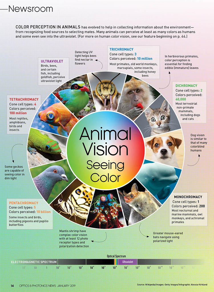
This chart represents the first defined quantitative link between distributions of wavelengths in the electromagnetic visible spectrum, and physiologically perceived colors in human color vision. Or basically, the range of color a typical human eye can perceive through visible light.
Note that while the human perception is quite wide, and generally speaking biased towards greens (we are apes after all), the amount of colors available through nature, generated through light reflection, tend to be a much smaller section. This is defined by the Pointer’s Chart.
In short. Color gamut is a representation of color coverage, used to describe data stored in images against available hardware and viewer technologies.
The CIE 1931 standard has been replaced by a CIE 1976 standard. Below we can see the significance of this.
People have observed that the biggest issue with CIE 1931 is the lack of uniformity with chromaticity, the three dimension color space in rectangular coordinates is not visually uniformed.
The CIE 1976 (also called CIELUV) was created by the CIE in 1976. It was put forward in an attempt to provide a more uniform color spacing than CIE 1931 for colors at approximately the same luminance
The CIE 1976 standard colour space is more linear and variations in perceived colour between different people has also been reduced. The disproportionately large green-turquoise area in CIE 1931, which cannot be generated with existing computer screens, has been reduced.
If we move from CIE 1931 to the CIE 1976 standard colour space we can see that the improvements made in the gamut for the “new” iPad screen (as compared to the “old” iPad 2) are more evident in the CIE 1976 colour space than in the CIE 1931 colour space, particularly in the blues from aqua to deep blue.
Despite its age, CIE 1931, named for the year of its adoption, remains a well-worn and familiar shorthand throughout the display industry. CIE 1931 is the primary language of customers. When a customer says that their current display “can do 72% of NTSC,” they implicitly mean 72% of NTSC 1953 color gamut as mapped against CIE 1931.
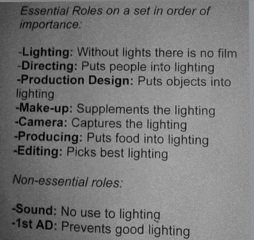
“Not every light performs the same way. Lights and lighting are tricky to handle. You have to plan for every circumstance. But the good news is, lighting can be adjusted. Let’s look at different factors that affect lighting in every scene you shoot. “
Use CRI, Luminous Efficacy and color temperature controls to match your needs.
Color Temperature Color temperature describes the “color” of white light by a light source radiated by a perfect black body at a given temperature measured in degrees Kelvin
CRI “The Color Rendering Index is a measurement of how faithfully a light source reveals the colors of whatever it illuminates, it describes the ability of a light source to reveal the color of an object, as compared to the color a natural light source would provide. The highest possible CRI is 100. A CRI of 100 generally refers to a perfect black body, like a tungsten light source or the sun. “
Spectralon is a teflon-based pressed powderthat comes closest to being a pure Lambertian diffuse material that reflects 100% of all light. If we take an HDR photograph of the Spectralon alongside the material to be measured, we can derive thediffuse albedo of that material.
The process to capture diffuse reflectance is very similar to the one outlined by Hable.
1. We put a linear polarizing filter in front of the camera lens and a second linear polarizing filterin front of a modeling light or a flash such that the two filters are oriented perpendicular to eachother, i.e. cross polarized.
2. We place Spectralon close to and parallel with the material we are capturing and take brack-eted shots of the setup7. Typically, we’ll take nine photographs, from -4EV to +4EV in 1EVincrements.
3. We convert the bracketed shots to a linear HDR image. We found that many HDR packagesdo not produce an HDR image in which the pixel values are linear. PTGui is an example of apackage which does generate a linear HDR image. At this point, because of the cross polarization,the image is one of surface diffuse response.
4. We open the file in Photoshop and normalize the image by color picking the Spectralon, filling anew layer with that color and setting that layer to “Divide”. This sets the Spectralon to 1 in theimage. All other color values are relative to this so we can consider them as diffuse albedo.
ACES 2.0 is the second major release of the components that make up the ACES system. The most significant change is a new suite of rendering transforms whose design was informed by collected feedback and requests from users of ACES 1. The changes aim to improve the appearance of perceived artifacts and to complete previously unfinished components of the system, resulting in a more complete, robust, and consistent product.
Highlights of the key changes in ACES 2.0 are as follows:
New output transforms, including:
A less aggressive tone scale
More intuitive controls to create custom outputs to non-standard displays
Robust gamut mapping to improve perceptual uniformity
Improved performance of the inverse transforms
Enhanced AMF specification
An updated specification for ACES Transform IDs
OpenEXR compression recommendations
Enhanced tools for generating Input Transforms and recommended procedures for characterizing prosumer cameras
Look Transform Library
Expanded documentation
Rendering Transform
The most substantial change in ACES 2.0 is a complete redesign of the rendering transform.
ACES 2.0 was built as a unified system, rather than through piecemeal additions. Different deliverable outputs “match” better and making outputs to display setups other than the provided presets is intended to be user-driven. The rendering transforms are less likely to produce undesirable artifacts “out of the box”, which means less time can be spent fixing problematic images and more time making pictures look the way you want.
Key design goals
Improve consistency of tone scale and provide an easy to use parameter to allow for outputs between preset dynamic ranges
Minimize hue skews across exposure range in a region of same hue
Unify for structural consistency across transform type
Easy to use parameters to create outputs other than the presets
Robust gamut mapping to improve harsh clipping artifacts
Fill extents of output code value cube (where appropriate and expected)
Invertible – not necessarily reversible, but Output > ACES > Output round-trip should be possible
Accomplish all of the above while maintaining an acceptable “out-of-the box” rendering
IES profiles are useful for creating life-like lighting, as they can represent the physical distribution of light from any light source.
The IES format was created by the Illumination Engineering Society, and most lighting manufacturers provide IES profile for the lights they manufacture.
An exposure stop is a unit measurement of Exposure as such it provides a universal linear scale to measure the increase and decrease in light, exposed to the image sensor, due to changes in shutter speed, iso and f-stop.
+-1 stop is a doubling or halving of the amount of light let in when taking a photo
1 EV (exposure value) is just another way to say one stop of exposure change.
Same applies to shutter speed, iso and aperture.
Doubling or halving your shutter speed produces an increase or decrease of 1 stop of exposure.
Doubling or halving your iso speed produces an increase or decrease of 1 stop of exposure.
import math,sys

def Exposure2Intensity(exposure):
    exp = float(exposure)
    result = math.pow(2,exp)
    print(result)

Exposure2Intensity(0)

def Intensity2Exposure(intensity):
    inarg = float(intensity)

    if inarg == 0:
        print("Exposure of zero intensity is undefined.")
        return

    if inarg < 1e-323:
        inarg = max(inarg, 1e-323)
        print("Exposure of negative intensities is undefined. Clamping to a very small value instead (1e-323)")

    result = math.log(inarg, 2)
    print(result)

Intensity2Exposure(0.1)
Why Exposure?
Exposure is a stop value that multiplies the intensity by 2 to the power of the stop. Increasing exposure by 1 results in double the amount of light.
Artists think in “stops.” Doubling or halving brightness is easy math and common in grading and look-dev. Exposure counts doublings in whole stops:
+1 stop = ×2 brightness
−1 stop = ×0.5 brightness
This gives perceptually even controls across both bright and dark values.
Why Intensity?
Intensity is linear. It’s what render engines and compositors expect when:
Summing values
Averaging pixels
Multiplying or filtering pixel data
Use intensity when you need the actual math on pixel/light data.
Formulas (from your Python)
Intensity from exposure: intensity = 2**exposure
Exposure from intensity: exposure = log₂(intensity)
Guardrails:
Intensity must be > 0 to compute exposure.
If intensity = 0 → exposure is undefined.
Clamp tiny values (e.g. 1e−323) before using log₂.
Use Exposure (stops) when…
You want artist-friendly sliders (−5…+5 stops)
Adjusting look-dev or grading in even stops
Matching plates with quick ±1 stop tweaks
Tweening brightness changes smoothly across ranges
Use Intensity (linear) when…
Storing raw pixel/light values
Multiplying textures or lights by a gain
Performing sums, averages, and filters
Feeding values to render engines expecting linear data
Examples
+2 stops → 2**2 = 4.0 (×4)
+1 stop → 2**1 = 2.0 (×2)
0 stop → 2**0 = 1.0 (×1)
−1 stop → 2**(−1) = 0.5 (×0.5)
−2 stops → 2**(−2) = 0.25 (×0.25)
Intensity 0.1 → exposure = log₂(0.1) ≈ −3.32
Rule of thumb
Think in stops (exposure) for controls and matching. Compute in linear (intensity) for rendering and math.
DISCLAIMER – Links and images on this website may be protected by the respective owners’ copyright. All data submitted by users through this site shall be treated as freely available to share.