


COMPOSITION
DESIGN
-
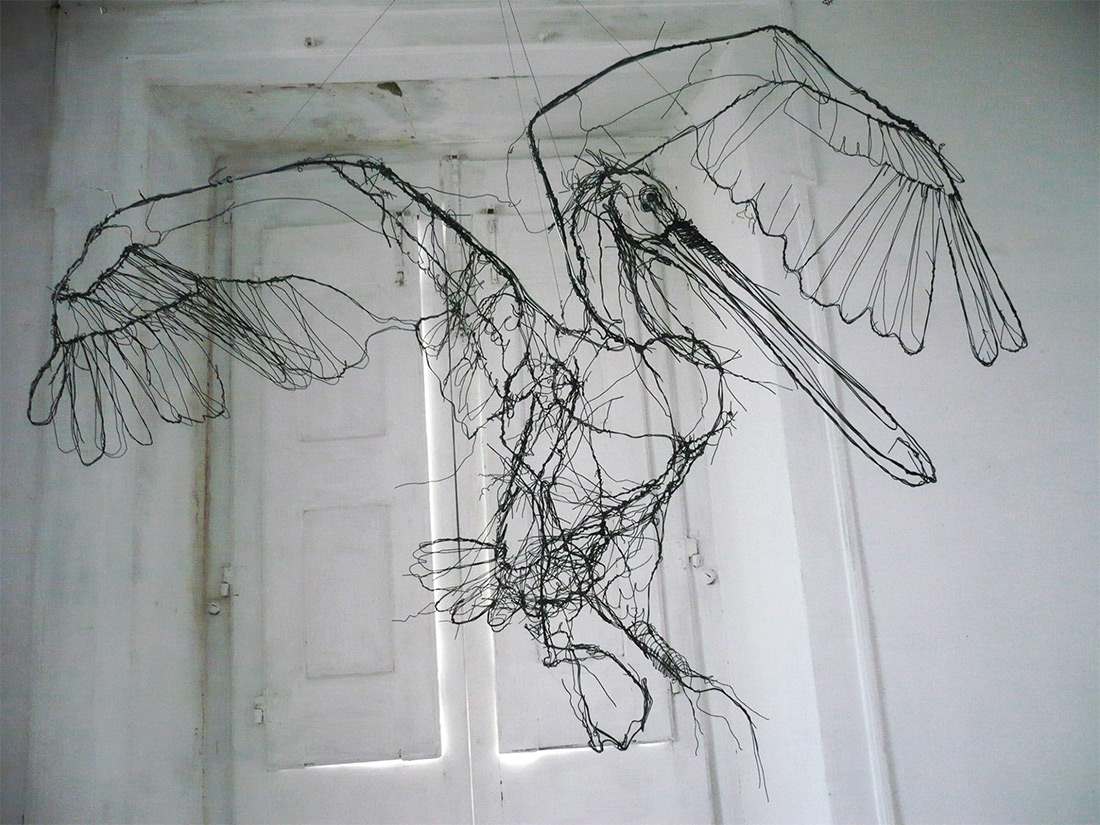
Goga Tandashvili – bas-relief master
Read more: Goga Tandashvili – bas-relief master@moltenimmersiveart Goga Tandashvili is a master of the art of Bas-Relief. Using this technique, he creates stunning figures that are slightly raised from a flat surface, bringing scenes inspired by the natural world to life. #Art #Artists #GogaTandashvili #BasReliefSculpture #ArtInspiredByNature #ImpressionistArt #BasRelief #Sculptures #Sculptor #Molten #MoltenArt #MoltenImmersiveArt #MoltenAffect #Curation #Curator #ArtCuration #ArtCurator #DorothyDiStefano ♬ original sound – Molten Immersive Art -
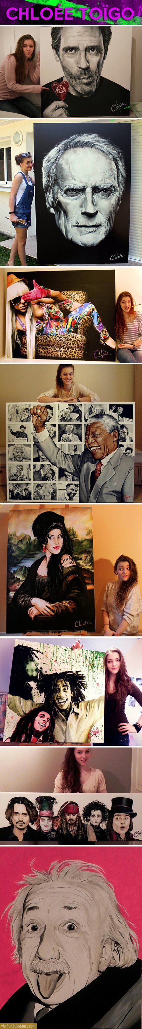
Mania Carta – Photorealistic Characters Made in Blender
Read more: Mania Carta – Photorealistic Characters Made in BlenderManiacarta is an Artist based in Tokyo, her Artworks are unique and she strive to create the best characters that have soul in the World.
https://80.lv/articles/marvelous-photorealistic-characters-made-in-blender-by-mania-carta/
https://www.instagram.com/mania_carta/


COLOR
-
Composition – cinematography Cheat Sheet
Read more: Composition – cinematography Cheat Sheet
Where is our eye attracted first? Why?
Size. Focus. Lighting. Color.
Size. Mr. White (Harvey Keitel) on the right.
Focus. He’s one of the two objects in focus.
Lighting. Mr. White is large and in focus and Mr. Pink (Steve Buscemi) is highlighted by
a shaft of light.
Color. Both are black and white but the read on Mr. White’s shirt now really stands out.
(more…)
What type of lighting? -
OLED vs QLED – What TV is better?
Read more: OLED vs QLED – What TV is better?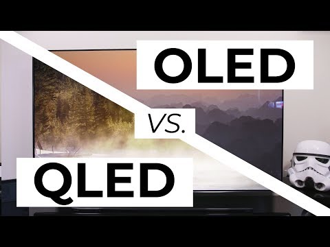
Supported by LG, Philips, Panasonic and Sony sell the OLED system TVs.
OLED stands for “organic light emitting diode.”
It is a fundamentally different technology from LCD, the major type of TV today.
OLED is “emissive,” meaning the pixels emit their own light.Samsung is branding its best TVs with a new acronym: “QLED”
QLED (according to Samsung) stands for “quantum dot LED TV.”
It is a variation of the common LED LCD, adding a quantum dot film to the LCD “sandwich.”
QLED, like LCD, is, in its current form, “transmissive” and relies on an LED backlight.OLED is the only technology capable of absolute blacks and extremely bright whites on a per-pixel basis. LCD definitely can’t do that, and even the vaunted, beloved, dearly departed plasma couldn’t do absolute blacks.
QLED, as an improvement over OLED, significantly improves the picture quality. QLED can produce an even wider range of colors than OLED, which says something about this new tech. QLED is also known to produce up to 40% higher luminance efficiency than OLED technology. Further, many tests conclude that QLED is far more efficient in terms of power consumption than its predecessor, OLED.
(more…) -
Light and Matter : The 2018 theory of Physically-Based Rendering and Shading by Allegorithmic
Read more: Light and Matter : The 2018 theory of Physically-Based Rendering and Shading by Allegorithmicacademy.substance3d.com/courses/the-pbr-guide-part-1
academy.substance3d.com/courses/the-pbr-guide-part-2

 Local copy:
-
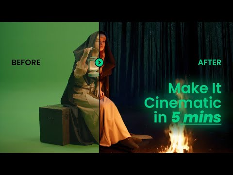
About green screens
Read more: About green screenshackaday.com/2015/02/07/how-green-screen-worked-before-computers/
www.newtek.com/blog/tips/best-green-screen-materials/
www.chromawall.com/blog//chroma-key-green

Chroma Key Green, the color of green screens is also known as Chroma Green and is valued at approximately 354C in the Pantone color matching system (PMS).
Chroma Green can be broken down in many different ways. Here is green screen green as other values useful for both physical and digital production:
Green Screen as RGB Color Value: 0, 177, 64
Green Screen as CMYK Color Value: 81, 0, 92, 0
Green Screen as Hex Color Value: #00b140
Green Screen as Websafe Color Value: #009933Chroma Key Green is reasonably close to an 18% gray reflectance.
Illuminate your green screen with an uniform source with less than 2/3 EV variation.
The level of brightness at any given f-stop should be equivalent to a 90% white card under the same lighting. -
RawTherapee – a free, open source, cross-platform raw image and HDRi processing program
Read more: RawTherapee – a free, open source, cross-platform raw image and HDRi processing program5.10 of this tool includes excellent tools to clean up cr2 and cr3 used on set to support HDRI processing.
Converting raw to AcesCG 32 bit tiffs with metadata.


LIGHTING
-
StudioBinder.com – CRI color rendering index
Read more: StudioBinder.com – CRI color rendering indexwww.studiobinder.com/blog/what-is-color-rendering-index
“The Color Rendering Index is a measurement of how faithfully a light source reveals the colors of whatever it illuminates, it describes the ability of a light source to reveal the color of an object, as compared to the color a natural light source would provide. The highest possible CRI is 100. A CRI of 100 generally refers to a perfect black body, like a tungsten light source or the sun. ”


www.pixelsham.com/2021/04/28/types-of-film-lights-and-their-efficiency
-
Composition – These are the basic lighting techniques you need to know for photography and film
Read more: Composition – These are the basic lighting techniques you need to know for photography and film
http://www.diyphotography.net/basic-lighting-techniques-need-know-photography-film/
Amongst the basic techniques, there’s…
1- Side lighting – Literally how it sounds, lighting a subject from the side when they’re faced toward you
2- Rembrandt lighting – Here the light is at around 45 degrees over from the front of the subject, raised and pointing down at 45 degrees
3- Back lighting – Again, how it sounds, lighting a subject from behind. This can help to add drama with silouettes
4- Rim lighting – This produces a light glowing outline around your subject
5- Key light – The main light source, and it’s not necessarily always the brightest light source
6- Fill light – This is used to fill in the shadows and provide detail that would otherwise be blackness
7- Cross lighting – Using two lights placed opposite from each other to light two subjects
-
What is the Light Field?
Read more: What is the Light Field?http://lightfield-forum.com/what-is-the-lightfield/
The light field consists of the total of all light rays in 3D space, flowing through every point and in every direction.
How to Record a Light Field
- a single, robotically controlled camera
- a rotating arc of cameras
- an array of cameras or camera modules
- a single camera or camera lens fitted with a microlens array


-
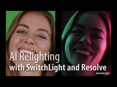
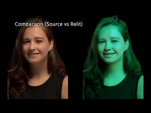
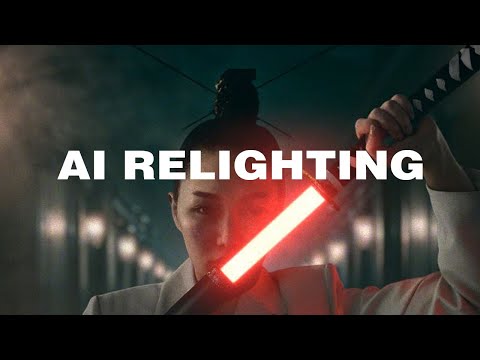
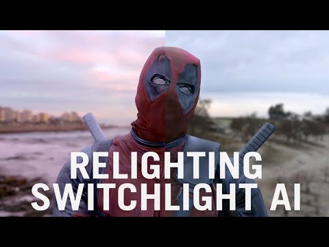
Beeble Switchlight’s Plugin for Foundry Nuke
Read more: Beeble Switchlight’s Plugin for Foundry Nukehttps://www.cutout.pro/learn/beeble-switchlight/
https://www.switchlight-api.beeble.ai/pricing
https://www.switchlight-api.beeble.ai
https://github.com/beeble-ai/SwitchLight-Studio
https://beeble.ai/terms-of-use
https://www.switchlight-api.beeble.ai/docs
-
Willem Zwarthoed – Aces gamut in VFX production pdf
Read more: Willem Zwarthoed – Aces gamut in VFX production pdfhttps://www.provideocoalition.com/color-management-part-12-introducing-aces/
Local copy:
https://www.slideshare.net/hpduiker/acescg-a-common-color-encoding-for-visual-effects-applications

![[gamma correction test]](http://www.madore.org/~david/misc/color/gammatest.png "sRGB gamma correction test")


COLLECTIONS
| Featured AI
| Design And Composition
| Explore posts
POPULAR SEARCHES
unreal | pipeline | virtual production | free | learn | photoshop | 360 | macro | google | nvidia | resolution | open source | hdri | real-time | photography basics | nuke
FEATURED POSTS
Social Links
DISCLAIMER – Links and images on this website may be protected by the respective owners’ copyright. All data submitted by users through this site shall be treated as freely available to share.
