


COMPOSITION
DESIGN
-
Mania Carta – Photorealistic Characters Made in Blender
Read more: Mania Carta – Photorealistic Characters Made in BlenderManiacarta is an Artist based in Tokyo, her Artworks are unique and she strive to create the best characters that have soul in the World.
https://80.lv/articles/marvelous-photorealistic-characters-made-in-blender-by-mania-carta/
https://www.instagram.com/mania_carta/


-
How to paint a boardgame miniatures
Read more: How to paint a boardgame miniatures
Steps:
- soap wash cleaning
- primer
- base-coat layer (black/white)
- detailing
- washing aka shade (could be done after highlighting)
- highlights aka dry brushing (could be done after washing)
- varnish (gloss/satin/matte)


COLOR
-
Colour – MacBeth Chart Checker Detection
Read more: Colour – MacBeth Chart Checker Detectiongithub.com/colour-science/colour-checker-detection
A Python package implementing various colour checker detection algorithms and related utilities.

-
Christopher Butler – Understanding the Eye-Mind Connection – Vision is a mental process
Read more: Christopher Butler – Understanding the Eye-Mind Connection – Vision is a mental processhttps://www.chrbutler.com/understanding-the-eye-mind-connection
The intricate relationship between the eyes and the brain, often termed the eye-mind connection, reveals that vision is predominantly a cognitive process. This understanding has profound implications for fields such as design, where capturing and maintaining attention is paramount. This essay delves into the nuances of visual perception, the brain’s role in interpreting visual data, and how this knowledge can be applied to effective design strategies.
This cognitive aspect of vision is evident in phenomena such as optical illusions, where the brain interprets visual information in a way that contradicts physical reality. These illusions underscore that what we “see” is not merely a direct recording of the external world but a constructed experience shaped by cognitive processes.
Understanding the cognitive nature of vision is crucial for effective design. Designers must consider how the brain processes visual information to create compelling and engaging visuals. This involves several key principles:
- Attention and Engagement
- Visual Hierarchy
- Cognitive Load Management
- Context and Meaning

-
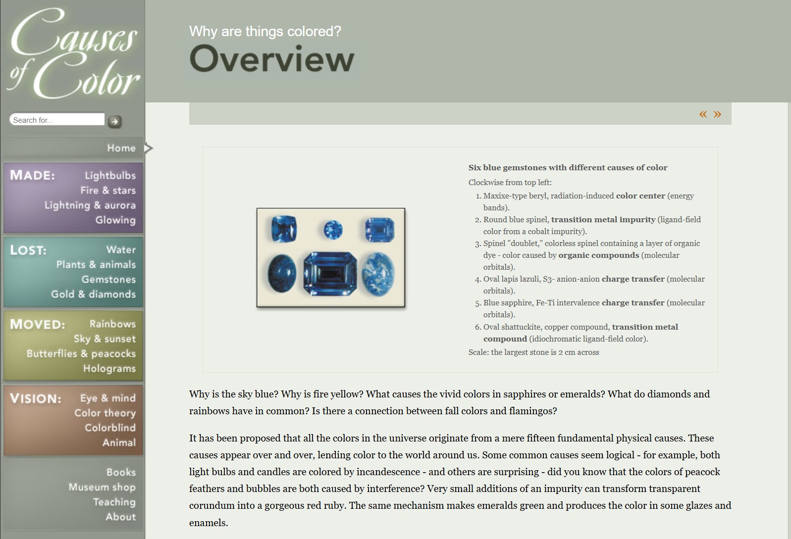
What causes color
Read more: What causes colorwww.webexhibits.org/causesofcolor/5.html
Water itself has an intrinsic blue color that is a result of its molecular structure and its behavior.
-
No one could see the colour blue until modern times
Read more: No one could see the colour blue until modern timeshttps://www.businessinsider.com/what-is-blue-and-how-do-we-see-color-2015-2

The way humans see the world… until we have a way to describe something, even something so fundamental as a colour, we may not even notice that something it’s there.
Ancient languages didn’t have a word for blue — not Greek, not Chinese, not Japanese, not Hebrew, not Icelandic cultures. And without a word for the colour, there’s evidence that they may not have seen it at all.
https://www.wnycstudios.org/story/211119-colorsEvery language first had a word for black and for white, or dark and light. The next word for a colour to come into existence — in every language studied around the world — was red, the colour of blood and wine.
After red, historically, yellow appears, and later, green (though in a couple of languages, yellow and green switch places). The last of these colours to appear in every language is blue.The only ancient culture to develop a word for blue was the Egyptians — and as it happens, they were also the only culture that had a way to produce a blue dye.
https://mymodernmet.com/shades-of-blue-color-history/True blue hues are rare in the natural world because synthesizing pigments that absorb longer-wavelength light (reds and yellows) while reflecting shorter-wavelength blue light requires exceptionally elaborate molecular structures—biochemical feats that most plants and animals simply don’t undertake.
When you gaze at a blueberry’s deep blue surface, you’re actually seeing structural coloration rather than a true blue pigment. A fine, waxy bloom on the berry’s skin contains nanostructures that preferentially scatter blue and violet light, giving the fruit its signature blue sheen even though its inherent pigment is reddish.
Similarly, many of nature’s most striking blues—like those of blue jays and morpho butterflies—arise not from blue pigments but from microscopic architectures in feathers or wing scales. These tiny ridges and air pockets manipulate incoming light so that blue wavelengths emerge most prominently, creating vivid, angle-dependent colors through scattering rather than pigment alone.
(more…) -
Photography basics: Lumens vs Candelas (candle) vs Lux vs FootCandle vs Watts vs Irradiance vs Illuminance
Read more: Photography basics: Lumens vs Candelas (candle) vs Lux vs FootCandle vs Watts vs Irradiance vs Illuminancehttps://www.translatorscafe.com/unit-converter/en-US/illumination/1-11/

The power output of a light source is measured using the unit of watts W. This is a direct measure to calculate how much power the light is going to drain from your socket and it is not relatable to the light brightness itself.
The amount of energy emitted from it per second. That energy comes out in a form of photons which we can crudely represent with rays of light coming out of the source. The higher the power the more rays emitted from the source in a unit of time.
Not all energy emitted is visible to the human eye, so we often rely on photometric measurements, which takes in account the sensitivity of human eye to different wavelenghts


Details in the post
(more…) -
VES Cinematic Color – Motion-Picture Color Management
Read more: VES Cinematic Color – Motion-Picture Color ManagementThis paper presents an introduction to the color pipelines behind modern feature-film visual-effects and animation.
Authored by Jeremy Selan, and reviewed by the members of the VES Technology Committee including Rob Bredow, Dan Candela, Nick Cannon, Paul Debevec, Ray Feeney, Andy Hendrickson, Gautham Krishnamurti, Sam Richards, Jordan Soles, and Sebastian Sylwan.
-
Rec-2020 – TVs new color gamut standard used by Dolby Vision?
Read more: Rec-2020 – TVs new color gamut standard used by Dolby Vision?https://www.hdrsoft.com/resources/dri.html#bit-depth

The dynamic range is a ratio between the maximum and minimum values of a physical measurement. Its definition depends on what the dynamic range refers to.
For a scene: Dynamic range is the ratio between the brightest and darkest parts of the scene.
For a camera: Dynamic range is the ratio of saturation to noise. More specifically, the ratio of the intensity that just saturates the camera to the intensity that just lifts the camera response one standard deviation above camera noise.
For a display: Dynamic range is the ratio between the maximum and minimum intensities emitted from the screen.
The Dynamic Range of real-world scenes can be quite high — ratios of 100,000:1 are common in the natural world. An HDR (High Dynamic Range) image stores pixel values that span the whole tonal range of real-world scenes. Therefore, an HDR image is encoded in a format that allows the largest range of values, e.g. floating-point values stored with 32 bits per color channel. Another characteristics of an HDR image is that it stores linear values. This means that the value of a pixel from an HDR image is proportional to the amount of light measured by the camera.
For TVs HDR is great, but it’s not the only new TV feature worth discussing.
(more…) -
About green screens
Read more: About green screenshackaday.com/2015/02/07/how-green-screen-worked-before-computers/
www.newtek.com/blog/tips/best-green-screen-materials/
www.chromawall.com/blog//chroma-key-green

Chroma Key Green, the color of green screens is also known as Chroma Green and is valued at approximately 354C in the Pantone color matching system (PMS).
Chroma Green can be broken down in many different ways. Here is green screen green as other values useful for both physical and digital production:
Green Screen as RGB Color Value: 0, 177, 64
Green Screen as CMYK Color Value: 81, 0, 92, 0
Green Screen as Hex Color Value: #00b140
Green Screen as Websafe Color Value: #009933Chroma Key Green is reasonably close to an 18% gray reflectance.
Illuminate your green screen with an uniform source with less than 2/3 EV variation.
The level of brightness at any given f-stop should be equivalent to a 90% white card under the same lighting.


LIGHTING
-
Open Source Nvidia Omniverse
Read more: Open Source Nvidia Omniverseblogs.nvidia.com/blog/2019/03/18/omniverse-collaboration-platform/
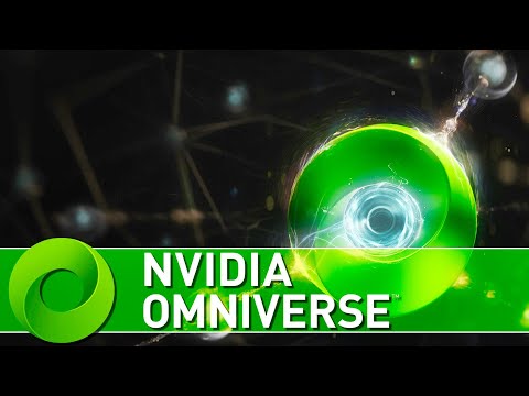
developer.nvidia.com/nvidia-omniverse
An open, Interactive 3D Design Collaboration Platform for Multi-Tool Workflows to simplify studio workflows for real-time graphics.
It supports Pixar’s Universal Scene Description technology for exchanging information about modeling, shading, animation, lighting, visual effects and rendering across multiple applications.
It also supports NVIDIA’s Material Definition Language, which allows artists to exchange information about surface materials across multiple tools.
With Omniverse, artists can see live updates made by other artists working in different applications. They can also see changes reflected in multiple tools at the same time.
For example an artist using Maya with a portal to Omniverse can collaborate with another artist using UE4 and both will see live updates of each others’ changes in their application.
-
HDRI Median Cut plugin
Read more: HDRI Median Cut pluginwww.hdrlabs.com/picturenaut/plugins.html

Note. The Median Cut algorithm is typically used for color quantization, which involves reducing the number of colors in an image while preserving its visual quality. It doesn’t directly provide a way to identify the brightest areas in an image. However, if you’re interested in identifying the brightest areas, you might want to look into other methods like thresholding, histogram analysis, or edge detection, through openCV for example.
Here is an openCV example:
(more…) -
Ethan Roffler interviews CG Supervisor Daniele Tosti
Read more: Ethan Roffler interviews CG Supervisor Daniele TostiEthan Roffler
I recently had the honor of interviewing this VFX genius and gained great insight into what it takes to work in the entertainment industry. Keep in mind, these questions are coming from an artist’s perspective but can be applied to any creative individual looking for some wisdom from a professional. So grab a drink, sit back, and enjoy this fun and insightful conversation.
Ethan
To start, I just wanted to say thank you so much for taking the time for this interview!Daniele
My pleasure.
When I started my career I struggled to find help. Even people in the industry at the time were not that helpful. Because of that, I decided very early on that I was going to do exactly the opposite. I spend most of my weekends talking or helping students. ;)Ethan
(more…)
That’s awesome! I have also come across the same struggle! Just a heads up, this will probably be the most informal interview you’ll ever have haha! Okay, so let’s start with a small introduction! -
Gamma correction
Read more: Gamma correction

http://www.normankoren.com/makingfineprints1A.html#Gammabox
https://en.wikipedia.org/wiki/Gamma_correction
http://www.photoscientia.co.uk/Gamma.htm
https://www.w3.org/Graphics/Color/sRGB.html
http://www.eizoglobal.com/library/basics/lcd_display_gamma/index.html
https://forum.reallusion.com/PrintTopic308094.aspx
Basically, gamma is the relationship between the brightness of a pixel as it appears on the screen, and the numerical value of that pixel. Generally Gamma is just about defining relationships.
Three main types:
– Image Gamma encoded in images
– Display Gammas encoded in hardware and/or viewing time
– System or Viewing Gamma which is the net effect of all gammas when you look back at a final image. In theory this should flatten back to 1.0 gamma.
(more…) -
Terminators and Iron Men: HDRI, Image-based lighting and physical shading at ILM – Siggraph 2010
Read more: Terminators and Iron Men: HDRI, Image-based lighting and physical shading at ILM – Siggraph 2010


COLLECTIONS
| Featured AI
| Design And Composition
| Explore posts
POPULAR SEARCHES
unreal | pipeline | virtual production | free | learn | photoshop | 360 | macro | google | nvidia | resolution | open source | hdri | real-time | photography basics | nuke
FEATURED POSTS
Social Links
DISCLAIMER – Links and images on this website may be protected by the respective owners’ copyright. All data submitted by users through this site shall be treated as freely available to share.
