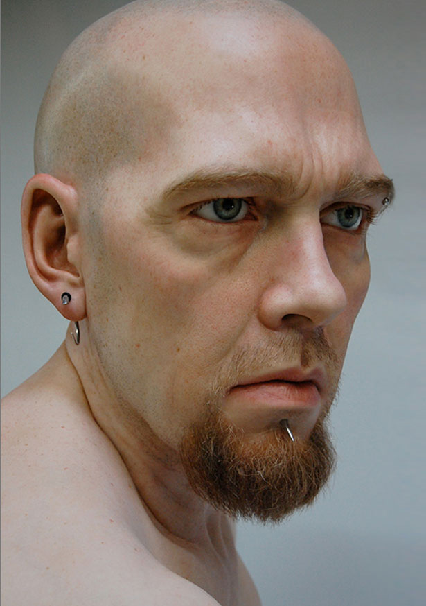
To measure the contrast ratio you will need a light meter. The process starts with you measuring the main source of light, or the key light.
Get a reading from the brightest area on the face of your subject. Then, measure the area lit by the secondary light, or fill light. To make sense of what you have just measured you have to understand that the information you have just gathered is in F-stops, a measure of light. With each additional F-stop, for example going one stop from f/1.4 to f/2.0, you create a doubling of light. The reverse is also true; moving one stop from f/8.0 to f/5.6 results in a halving of the light.
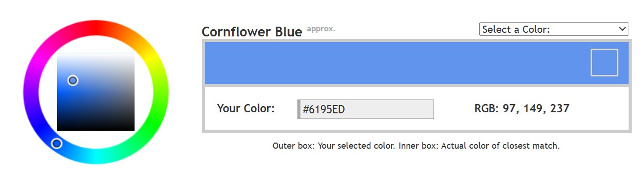
The way humans see the world… until we have a way to describe something, even something so fundamental as a colour, we may not even notice that something it’s there.
Ancient languages didn’t have a word for blue — not Greek, not Chinese, not Japanese, not Hebrew, not Icelandic cultures. And without a word for the colour, there’s evidence that they may not have seen it at all. https://www.wnycstudios.org/story/211119-colors
Every language first had a word for black and for white, or dark and light. The next word for a colour to come into existence — in every language studied around the world — was red, the colour of blood and wine. After red, historically, yellow appears, and later, green (though in a couple of languages, yellow and green switch places). The last of these colours to appear in every language is blue.
The only ancient culture to develop a word for blue was the Egyptians — and as it happens, they were also the only culture that had a way to produce a blue dye. https://mymodernmet.com/shades-of-blue-color-history/
True blue hues are rare in the natural world because synthesizing pigments that absorb longer-wavelength light (reds and yellows) while reflecting shorter-wavelength blue light requires exceptionally elaborate molecular structures—biochemical feats that most plants and animals simply don’t undertake.
When you gaze at a blueberry’s deep blue surface, you’re actually seeing structural coloration rather than a true blue pigment. A fine, waxy bloom on the berry’s skin contains nanostructures that preferentially scatter blue and violet light, giving the fruit its signature blue sheen even though its inherent pigment is reddish.
Similarly, many of nature’s most striking blues—like those of blue jays and morpho butterflies—arise not from blue pigments but from microscopic architectures in feathers or wing scales. These tiny ridges and air pockets manipulate incoming light so that blue wavelengths emerge most prominently, creating vivid, angle-dependent colors through scattering rather than pigment alone.
5.10 of this tool includes excellent tools to clean up cr2 and cr3 used on set to support HDRI processing.
Converting raw to AcesCG 32 bit tiffs with metadata.
RGBW (RGB + White) LED strip uses a 4-in-1 LED chip made up of red, green, blue, and white.
RGBWW (RGB + White + Warm White) LED strip uses either a 5-in-1 LED chip with red, green, blue, white, and warm white for color mixing. The only difference between RGBW and RGBWW is the intensity of the white color. The term RGBCCT consists of RGB and CCT. CCT (Correlated Color Temperature) means that the color temperature of the led strip light can be adjusted to change between warm white and white. Thus, RGBWW strip light is another name of RGBCCT strip.
RGBCW is the acronym for Red, Green, Blue, Cold, and Warm. These 5-in-1 chips are used in supper bright smart LED lighting products
The goals of lighting in 3D computer graphics are more or less the same as those of real world lighting.
Lighting serves a basic function of bringing out, or pushing back the shapes of objects visible from the camera’s view.
It gives a two-dimensional image on the monitor an illusion of the third dimension-depth.
But it does not just stop there. It gives an image its personality, its character. A scene lit in different ways can give a feeling of happiness, of sorrow, of fear etc., and it can do so in dramatic or subtle ways. Along with personality and character, lighting fills a scene with emotion that is directly transmitted to the viewer.
Trying to simulate a real environment in an artificial one can be a daunting task. But even if you make your 3D rendering look absolutely photo-realistic, it doesn’t guarantee that the image carries enough emotion to elicit a “wow” from the people viewing it.
Making 3D renderings photo-realistic can be hard. Putting deep emotions in them can be even harder. However, if you plan out your lighting strategy for the mood and emotion that you want your rendering to express, you make the process easier for yourself.
Each light source can be broken down in to 4 distinct components and analyzed accordingly.
· Intensity
· Direction
· Color
· Size
The overall thrust of this writing is to produce photo-realistic images by applying good lighting techniques.
DISCLAIMER – Links and images on this website may be protected by the respective owners’ copyright. All data submitted by users through this site shall be treated as freely available to share.