


COMPOSITION
-
Photography basics: Camera Aspect Ratio, Sensor Size and Depth of Field – resolutions
Read more: Photography basics: Camera Aspect Ratio, Sensor Size and Depth of Field – resolutionshttp://www.shutterangle.com/2012/cinematic-look-aspect-ratio-sensor-size-depth-of-field/
http://www.shutterangle.com/2012/film-video-aspect-ratio-artistic-choice/


DESIGN
-
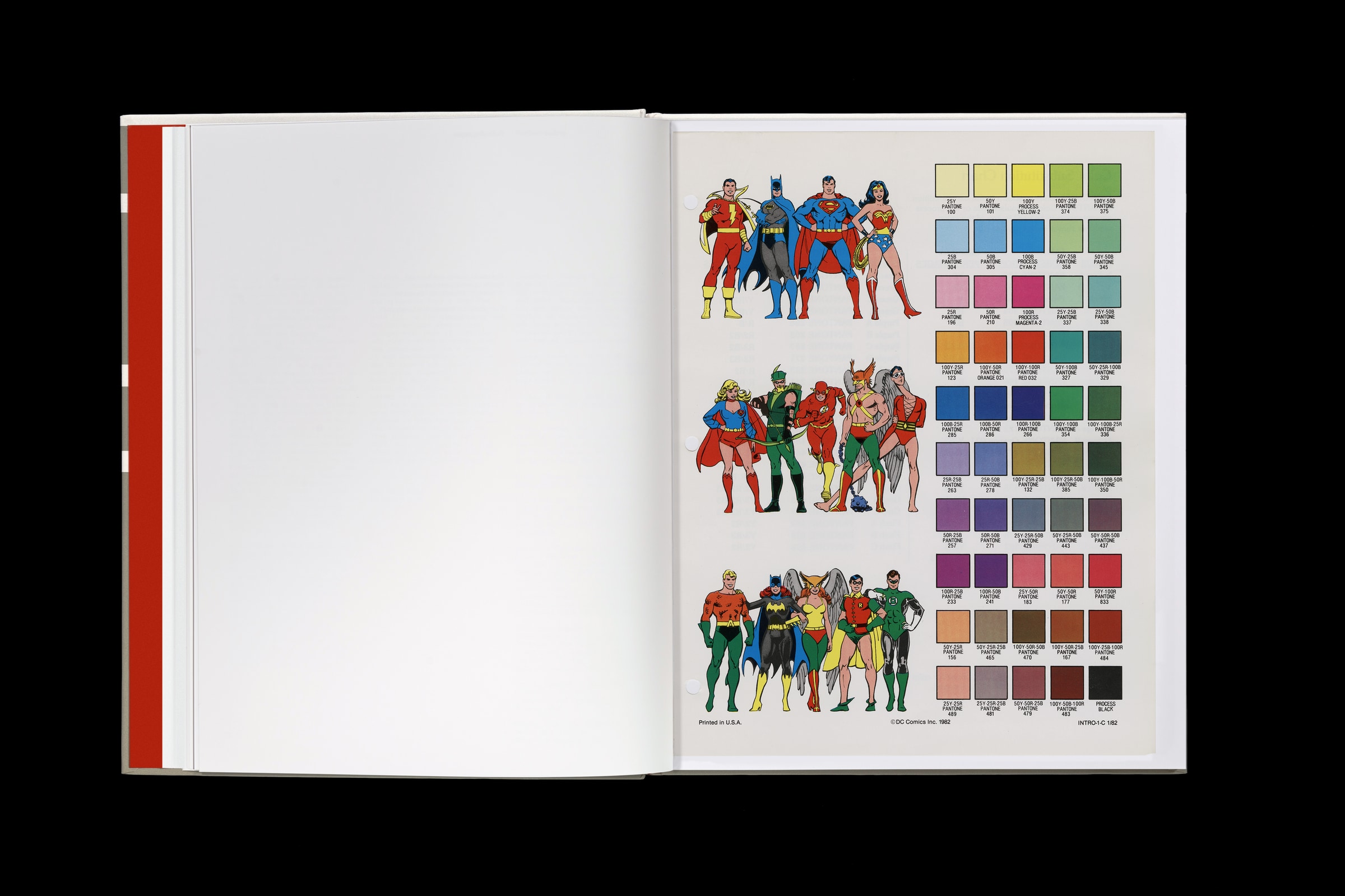
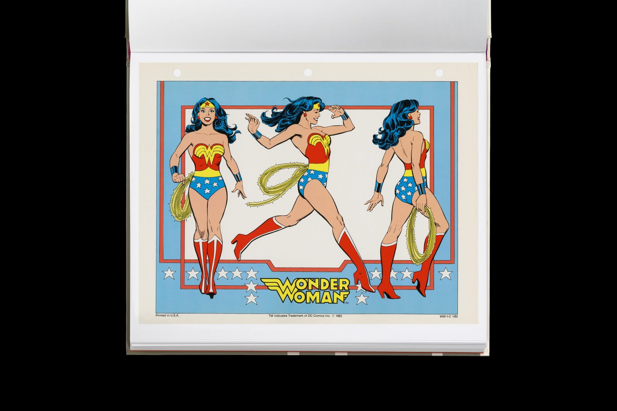
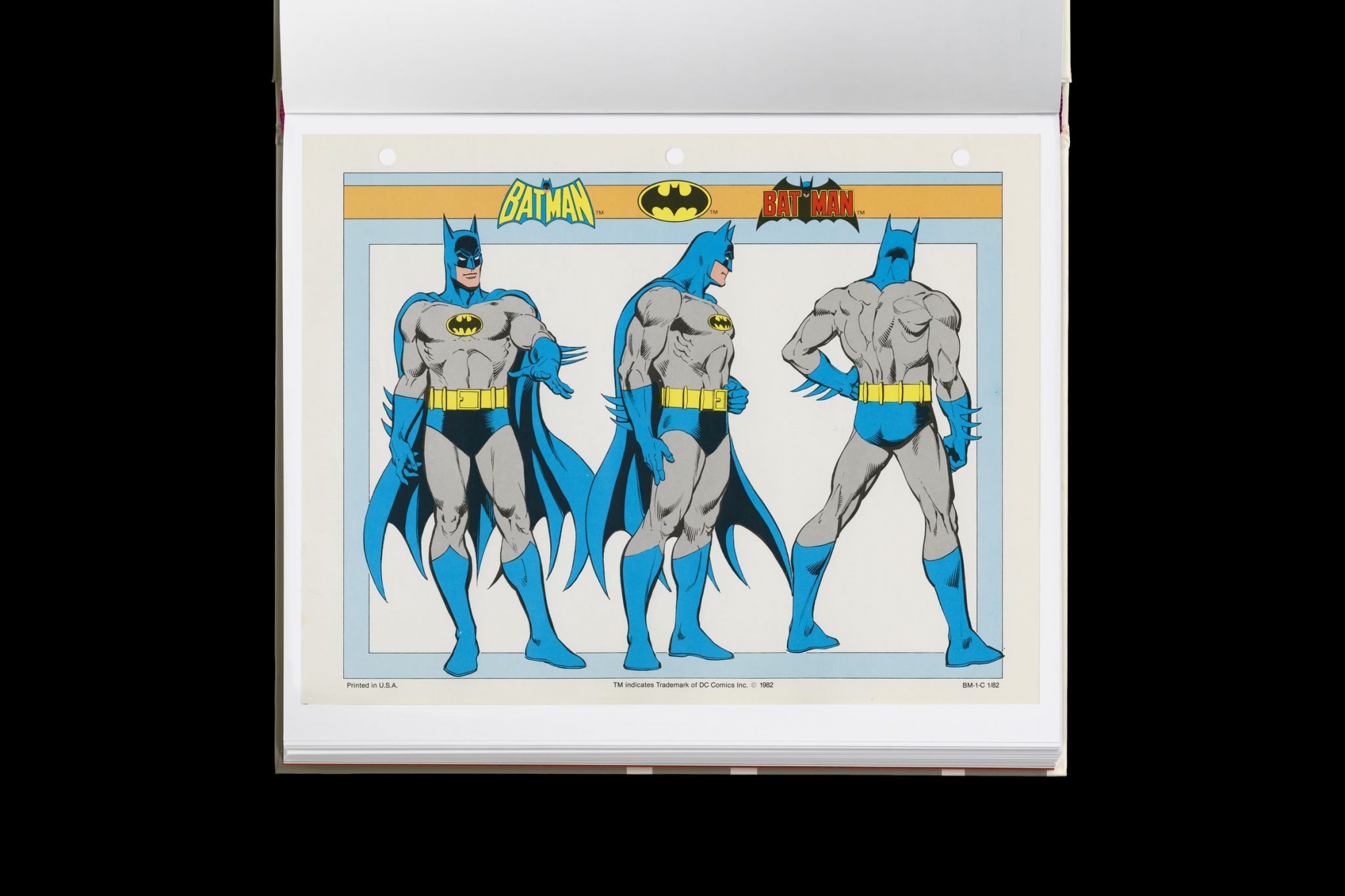
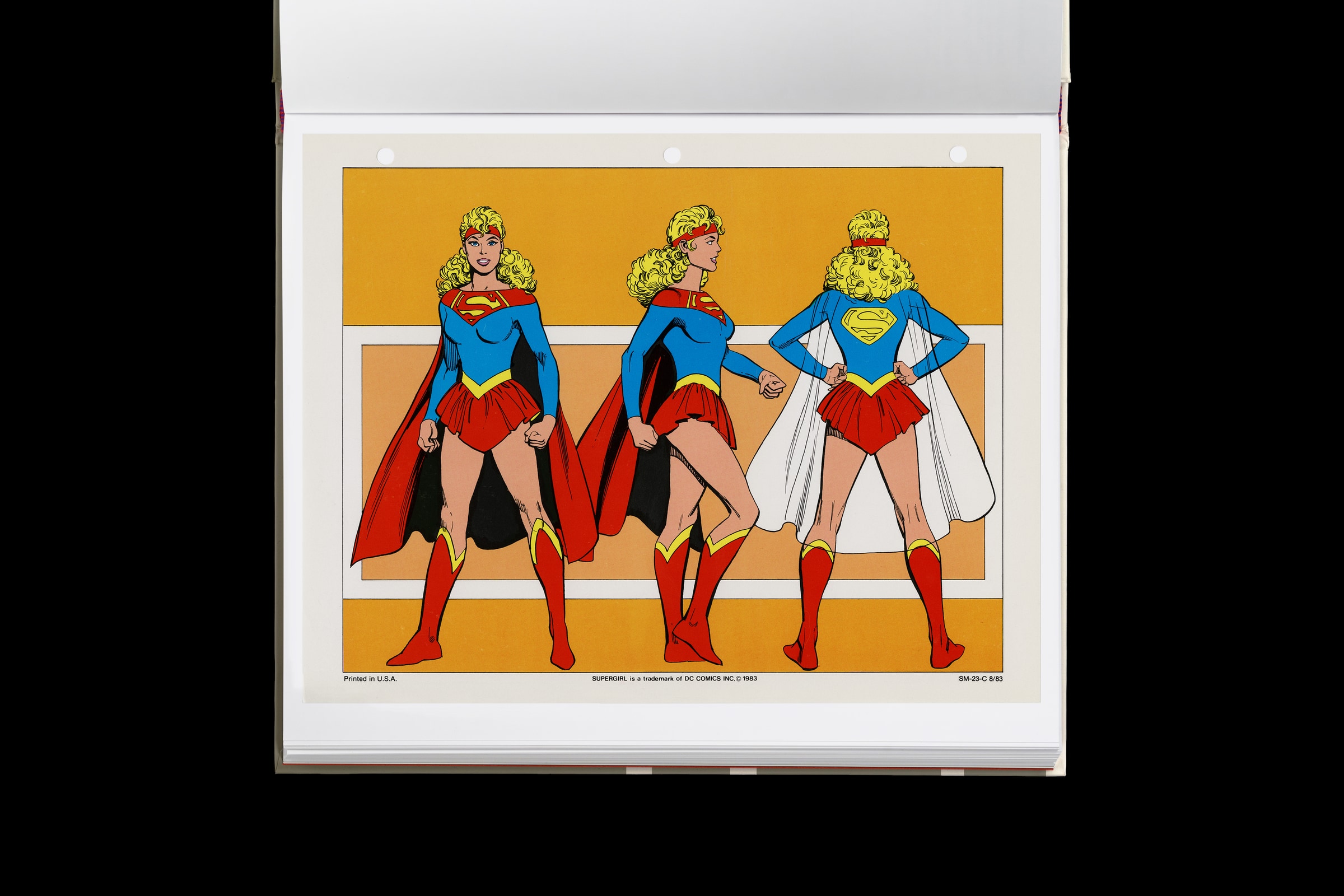
This legendary DC Comics style guide was nearly lost for years – now you can buy it
Read more: This legendary DC Comics style guide was nearly lost for years – now you can buy ithttps://www.fastcompany.com/91133306/dc-comics-style-guide-was-lost-for-years-now-you-can-buy-it
Reproduced from a rare original copy, the book features over 165 highly-detailed scans of the legendary art by José Luis García-López, with an introduction by Paul Levitz, former president of DC Comics.
https://standardsmanual.com/products/1982-dc-comics-style-guide
-
Mania Carta – Photorealistic Characters Made in Blender
Read more: Mania Carta – Photorealistic Characters Made in BlenderManiacarta is an Artist based in Tokyo, her Artworks are unique and she strive to create the best characters that have soul in the World.
https://80.lv/articles/marvelous-photorealistic-characters-made-in-blender-by-mania-carta/
https://www.instagram.com/mania_carta/


COLOR
-
VES Cinematic Color – Motion-Picture Color Management
Read more: VES Cinematic Color – Motion-Picture Color ManagementThis paper presents an introduction to the color pipelines behind modern feature-film visual-effects and animation.
Authored by Jeremy Selan, and reviewed by the members of the VES Technology Committee including Rob Bredow, Dan Candela, Nick Cannon, Paul Debevec, Ray Feeney, Andy Hendrickson, Gautham Krishnamurti, Sam Richards, Jordan Soles, and Sebastian Sylwan.
-
Rec-2020 – TVs new color gamut standard used by Dolby Vision?
Read more: Rec-2020 – TVs new color gamut standard used by Dolby Vision?https://www.hdrsoft.com/resources/dri.html#bit-depth

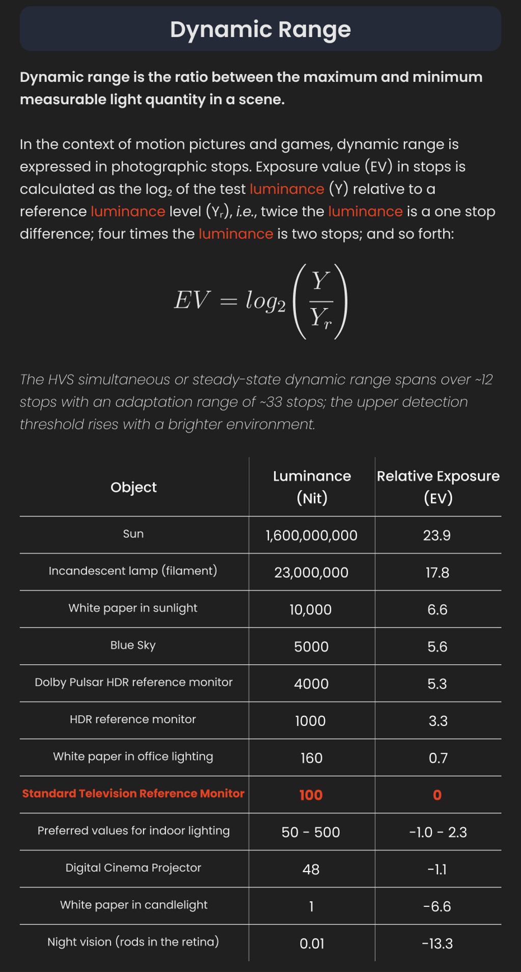
The dynamic range is a ratio between the maximum and minimum values of a physical measurement. Its definition depends on what the dynamic range refers to.
For a scene: Dynamic range is the ratio between the brightest and darkest parts of the scene.
For a camera: Dynamic range is the ratio of saturation to noise. More specifically, the ratio of the intensity that just saturates the camera to the intensity that just lifts the camera response one standard deviation above camera noise.
For a display: Dynamic range is the ratio between the maximum and minimum intensities emitted from the screen.
The Dynamic Range of real-world scenes can be quite high — ratios of 100,000:1 are common in the natural world. An HDR (High Dynamic Range) image stores pixel values that span the whole tonal range of real-world scenes. Therefore, an HDR image is encoded in a format that allows the largest range of values, e.g. floating-point values stored with 32 bits per color channel. Another characteristics of an HDR image is that it stores linear values. This means that the value of a pixel from an HDR image is proportional to the amount of light measured by the camera.
For TVs HDR is great, but it’s not the only new TV feature worth discussing.
(more…) -
Anders Langlands – Render Color Spaces
Read more: Anders Langlands – Render Color Spaceshttps://www.colour-science.org/anders-langlands/
This page compares images rendered in Arnold using spectral rendering and different sets of colourspace primaries: Rec.709, Rec.2020, ACES and DCI-P3. The SPD data for the GretagMacbeth Color Checker are the measurements of Noburu Ohta, taken from Mansencal, Mauderer and Parsons (2014) colour-science.org.

-
mmColorTarget – Nuke Gizmo for color matching a MacBeth chart
Read more: mmColorTarget – Nuke Gizmo for color matching a MacBeth charthttps://www.marcomeyer-vfx.de/posts/2014-04-11-mmcolortarget-nuke-gizmo/
https://www.marcomeyer-vfx.de/posts/mmcolortarget-nuke-gizmo/
https://vimeo.com/9.1652466e+07
https://www.nukepedia.com/gizmos/colour/mmcolortarget


LIGHTING
-
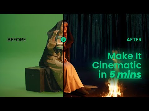
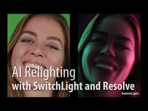
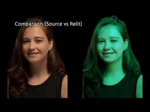
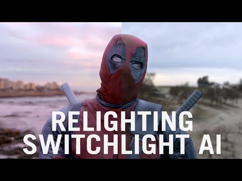
Beeble Switchlight’s Plugin for Foundry Nuke
Read more: Beeble Switchlight’s Plugin for Foundry Nukehttps://www.cutout.pro/learn/beeble-switchlight/
https://www.switchlight-api.beeble.ai/pricing
https://www.switchlight-api.beeble.ai
https://github.com/beeble-ai/SwitchLight-Studio
https://beeble.ai/terms-of-use
https://www.switchlight-api.beeble.ai/docs
-
HDRI Resources
Read more: HDRI ResourcesText2Light
- https://www.cgtrader.com/free-3d-models/exterior/other/10-free-hdr-panoramas-created-with-text2light-zero-shot
- https://frozenburning.github.io/projects/text2light/
- https://github.com/FrozenBurning/Text2Light
Royalty free links
- https://locationtextures.com/panoramas/
- http://www.noahwitchell.com/freebies
- https://polyhaven.com/hdris
- https://hdrmaps.com/
- https://www.ihdri.com/
- https://hdrihaven.com/
- https://www.domeble.com/
- http://www.hdrlabs.com/sibl/archive.html
- https://www.hdri-hub.com/hdrishop/hdri
- http://noemotionhdrs.net/hdrevening.html
- https://www.openfootage.net/hdri-panorama/
- https://www.zwischendrin.com/en/browse/hdri
Nvidia GauGAN360
-
DiffusionLight: HDRI Light Probes for Free by Painting a Chrome Ball
Read more: DiffusionLight: HDRI Light Probes for Free by Painting a Chrome Ballhttps://diffusionlight.github.io/
https://github.com/DiffusionLight/DiffusionLight
https://github.com/DiffusionLight/DiffusionLight?tab=MIT-1-ov-file#readme
https://colab.research.google.com/drive/15pC4qb9mEtRYsW3utXkk-jnaeVxUy-0S
“a simple yet effective technique to estimate lighting in a single input image. Current techniques rely heavily on HDR panorama datasets to train neural networks to regress an input with limited field-of-view to a full environment map. However, these approaches often struggle with real-world, uncontrolled settings due to the limited diversity and size of their datasets. To address this problem, we leverage diffusion models trained on billions of standard images to render a chrome ball into the input image. Despite its simplicity, this task remains challenging: the diffusion models often insert incorrect or inconsistent objects and cannot readily generate images in HDR format. Our research uncovers a surprising relationship between the appearance of chrome balls and the initial diffusion noise map, which we utilize to consistently generate high-quality chrome balls. We further fine-tune an LDR difusion model (Stable Diffusion XL) with LoRA, enabling it to perform exposure bracketing for HDR light estimation. Our method produces convincing light estimates across diverse settings and demonstrates superior generalization to in-the-wild scenarios.”

-
Aputure AL-F7 – dimmable Led Video Light, CRI95+, 3200-9500K
Read more: Aputure AL-F7 – dimmable Led Video Light, CRI95+, 3200-9500KHigh CRI of ≥95
256 LEDs with 45° beam angle
3200 to 9500K variable color temperature
1 to 100% Stepless Dimming, 1500 Lux Brightness at 3.3′
LCD Info Screen. Powered by an L-series battery, D-Tap, or USB-C
Because the light has a variable color range of 3200 to 9500K, when the light is set to 5500K (daylight balanced) both sets of LEDs are on at full, providing the maximum brightness from this fixture when compared to using the light at 3200 or 9500K.
The LCD screen provides information on the fixture’s output as well as the charge state of the battery. The screen also indicates whether the adjustment knob is controlling brightness or color temperature. To switch from brightness to CCT or CCT to brightness, just apply a short press to the adjustment knob.
The included cold shoe ball joint adapter enables mounting the light to your camera’s accessory shoe via the 1/4″-20 threaded hole on the fixture. In addition, the bottom of the cold shoe foot features a 3/8″-16 threaded hole, and includes a 3/8″-16 to 1/4″-20 reducing bushing.


-
How to Direct and Edit a Fight Scene for Rhythm and Pacing
Read more: How to Direct and Edit a Fight Scene for Rhythm and Pacingwww.premiumbeat.com/blog/directing-fight-scene-cinematography/
1- Frame the action
2- Stage the action
3- Use camera movements
4- Set a rhythm
5- Control the speed of the action


COLLECTIONS
| Featured AI
| Design And Composition
| Explore posts
POPULAR SEARCHES
unreal | pipeline | virtual production | free | learn | photoshop | 360 | macro | google | nvidia | resolution | open source | hdri | real-time | photography basics | nuke
FEATURED POSTS
-
GretagMacbeth Color Checker Numeric Values and Middle Gray
-
sRGB vs REC709 – An introduction and FFmpeg implementations
-
N8N.io – From Zero to Your First AI Agent in 25 Minutes
-
Black Forest Labs released FLUX.1 Kontext
-
Jesse Zumstein – Jobs in games
-
Kling 1.6 and competitors – advanced tests and comparisons
-
MiniTunes V1 – Free MP3 library app
-
Embedding frame ranges into Quicktime movies with FFmpeg
Social Links
DISCLAIMER – Links and images on this website may be protected by the respective owners’ copyright. All data submitted by users through this site shall be treated as freely available to share.
