slowmoVideo is an OpenSource program that creates slow-motion videos from your footage.
Slow motion cinematography is the result of playing back frames for a longer duration than they were exposed. For example, if you expose 240 frames of film in one second, then play them back at 24 fps, the resulting movie is 10 times longer (slower) than the original filmed event….
Film cameras are relatively simple mechanical devices that allow you to crank up the speed to whatever rate the shutter and pull-down mechanism allow. Some film cameras can operate at 2,500 fps or higher (although film shot in these cameras often needs some readjustment in postproduction). Video, on the other hand, is always captured, recorded, and played back at a fixed rate, with a current limit around 60fps. This makes extreme slow motion effects harder to achieve (and less elegant) on video, because slowing down the video results in each frame held still on the screen for a long time, whereas with high-frame-rate film there are plenty of frames to fill the longer durations of time. On video, the slow motion effect is more like a slide show than smooth, continuous motion.
One obvious solution is to shoot film at high speed, then transfer it to video (a case where film still has a clear advantage, sorry George). Another possibility is to cross dissolve or blur from one frame to the next. This adds a smooth transition from one still frame to the next. The blur reduces the sharpness of the image, and compared to slowing down images shot at a high frame rate, this is somewhat of a cheat. However, there isn’t much you can do about it until video can be recorded at much higher rates. Of course, many film cameras can’t shoot at high frame rates either, so the whole super-slow-motion endeavor is somewhat specialized no matter what medium you are using. (There are some high speed digital cameras available now that allow you to capture lots of digital frames directly to your computer, so technology is starting to catch up with film. However, this feature isn’t going to appear in consumer camcorders any time soon.)
“Not every light performs the same way. Lights and lighting are tricky to handle. You have to plan for every circumstance. But the good news is, lighting can be adjusted. Let’s look at different factors that affect lighting in every scene you shoot. “
Use CRI, Luminous Efficacy and color temperature controls to match your needs.
Color Temperature Color temperature describes the “color” of white light by a light source radiated by a perfect black body at a given temperature measured in degrees Kelvin
CRI “The Color Rendering Index is a measurement of how faithfully a light source reveals the colors of whatever it illuminates, it describes the ability of a light source to reveal the color of an object, as compared to the color a natural light source would provide. The highest possible CRI is 100. A CRI of 100 generally refers to a perfect black body, like a tungsten light source or the sun. “
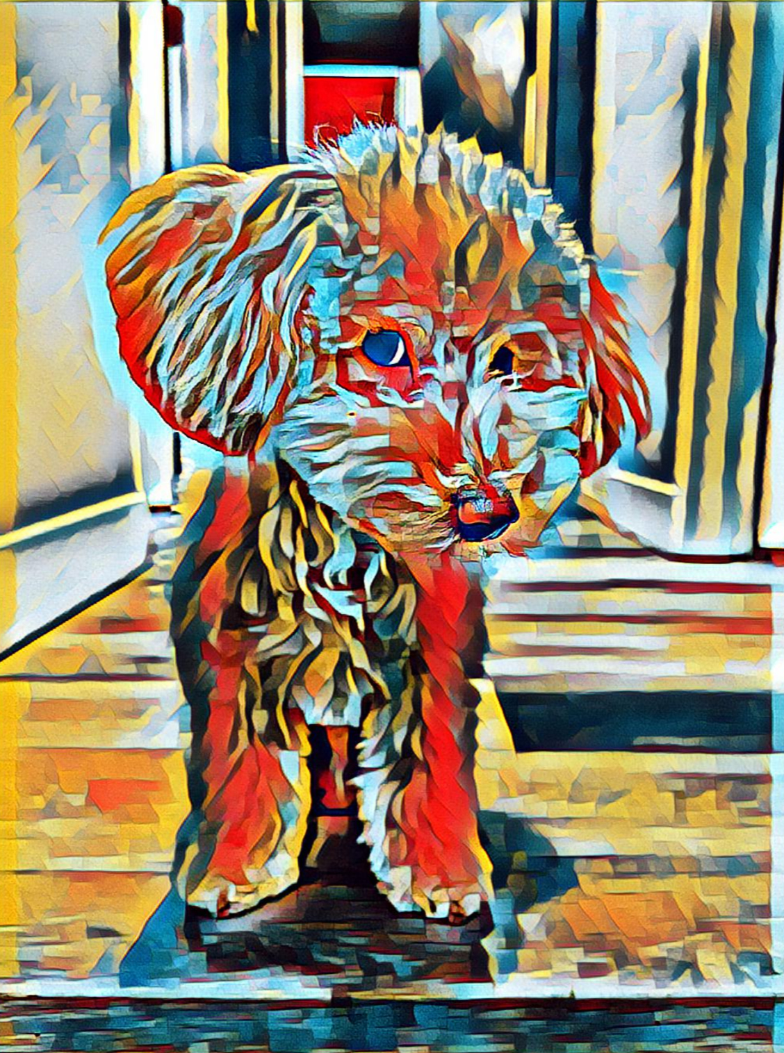
I was working an album cover last night and got these really cool images in midjourney so made a video out of it. Animated using Pika. Song made using Suno Full version on my bandcamp. It’s called Static.
“The Color Rendering Index is a measurement of how faithfully a light source reveals the colors of whatever it illuminates, it describes the ability of a light source to reveal the color of an object, as compared to the color a natural light source would provide. The highest possible CRI is 100. A CRI of 100 generally refers to a perfect black body, like a tungsten light source or the sun. ”
One problem with sRGB is that in a gradient between blue and white, it becomes a bit purple in the middle of the transition. That’s because sRGB really isn’t created to mimic how the eye sees colors; rather, it is based on how CRT monitors work. That means it works with certain frequencies of red, green, and blue, and also the non-linear coding called gamma. It’s a miracle it works as well as it does, but it’s not connected to color perception. When using those tools, you sometimes get surprising results, like purple in the gradient.
There were also attempts to create simple models matching human perception based on XYZ, but as it turned out, it’s not possible to model all color vision that way. Perception of color is incredibly complex and depends, among other things, on whether it is dark or light in the room and the background color it is against. When you look at a photograph, it also depends on what you think the color of the light source is. The dress is a typical example of color vision being very context-dependent. It is almost impossible to model this perfectly.
I based Oklab on two other color spaces, CIECAM16 and IPT. I used the lightness and saturation prediction from CIECAM16, which is a color appearance model, as a target. I actually wanted to use the datasets used to create CIECAM16, but I couldn’t find them.
IPT was designed to have better hue uniformity. In experiments, they asked people to match light and dark colors, saturated and unsaturated colors, which resulted in a dataset for which colors, subjectively, have the same hue. IPT has a few other issues but is the basis for hue in Oklab.
In the Munsell color system, colors are described with three parameters, designed to match the perceived appearance of colors: Hue, Chroma and Value. The parameters are designed to be independent and each have a uniform scale. This results in a color solid with an irregular shape. The parameters are designed to be independent and each have a uniform scale. This results in a color solid with an irregular shape. Modern color spaces and models, such as CIELAB, Cam16 and Björn Ottosson own Oklab, are very similar in their construction.
By far the most used color spaces today for color picking are HSL and HSV, two representations introduced in the classic 1978 paper “Color Spaces for Computer Graphics”. HSL and HSV designed to roughly correlate with perceptual color properties while being very simple and cheap to compute.
Today HSL and HSV are most commonly used together with the sRGB color space.
One of the main advantages of HSL and HSV over the different Lab color spaces is that they map the sRGB gamut to a cylinder. This makes them easy to use since all parameters can be changed independently, without the risk of creating colors outside of the target gamut.
The main drawback on the other hand is that their properties don’t match human perception particularly well.
Reconciling these conflicting goals perfectly isn’t possible, but given that HSV and HSL don’t use anything derived from experiments relating to human perception, creating something that makes a better tradeoff does not seem unreasonable.
With this new lightness estimate, we are ready to look into the construction of Okhsv and Okhsl.
ACES 2.0 is the second major release of the components that make up the ACES system. The most significant change is a new suite of rendering transforms whose design was informed by collected feedback and requests from users of ACES 1. The changes aim to improve the appearance of perceived artifacts and to complete previously unfinished components of the system, resulting in a more complete, robust, and consistent product.
Highlights of the key changes in ACES 2.0 are as follows:
New output transforms, including:
A less aggressive tone scale
More intuitive controls to create custom outputs to non-standard displays
Robust gamut mapping to improve perceptual uniformity
Improved performance of the inverse transforms
Enhanced AMF specification
An updated specification for ACES Transform IDs
OpenEXR compression recommendations
Enhanced tools for generating Input Transforms and recommended procedures for characterizing prosumer cameras
Look Transform Library
Expanded documentation
Rendering Transform
The most substantial change in ACES 2.0 is a complete redesign of the rendering transform.
ACES 2.0 was built as a unified system, rather than through piecemeal additions. Different deliverable outputs “match” better and making outputs to display setups other than the provided presets is intended to be user-driven. The rendering transforms are less likely to produce undesirable artifacts “out of the box”, which means less time can be spent fixing problematic images and more time making pictures look the way you want.
Key design goals
Improve consistency of tone scale and provide an easy to use parameter to allow for outputs between preset dynamic ranges
Minimize hue skews across exposure range in a region of same hue
Unify for structural consistency across transform type
Easy to use parameters to create outputs other than the presets
Robust gamut mapping to improve harsh clipping artifacts
Fill extents of output code value cube (where appropriate and expected)
Invertible – not necessarily reversible, but Output > ACES > Output round-trip should be possible
Accomplish all of the above while maintaining an acceptable “out-of-the box” rendering
A way to approximate complex lighting in ultra realistic renders.
All SH lighting techniques involve replacing parts of standard lighting equations with spherical functions that have been projected into frequency space using the spherical harmonics as a basis.
As Einstein showed us, light and matter and just aspects of the same thing. Matter is just frozen light. And light is matter on the move. Albert Einstein’s most famous equation says that energy and matter are two sides of the same coin. How does one become the other?
Relativity requires that the faster an object moves, the more mass it appears to have. This means that somehow part of the energy of the car’s motion appears to transform into mass. Hence the origin of Einstein’s equation. How does that happen? We don’t really know. We only know that it does.
Matter is 99.999999999999 percent empty space. Not only do the atom and solid matter consist mainly of empty space, it is the same in outer space
The quantum theory researchers discovered the answer: Not only do particles consist of energy, but so does the space between. This is the so-called zero-point energy. Therefore it is true: Everything consists of energy.
Energy is the basis of material reality. Every type of particle is conceived of as a quantum vibration in a field: Electrons are vibrations in electron fields, protons vibrate in a proton field, and so on. Everything is energy, and everything is connected to everything else through fields.
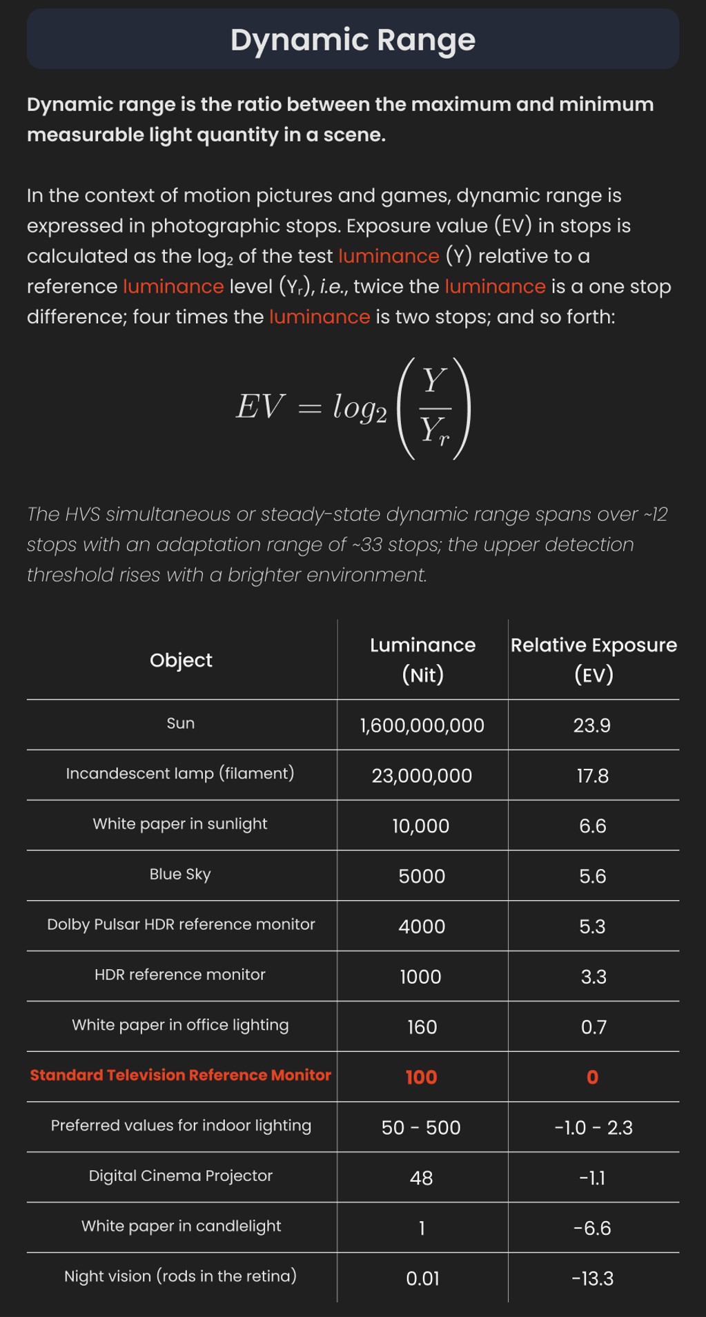
An exposure stop is a unit measurement of Exposure as such it provides a universal linear scale to measure the increase and decrease in light, exposed to the image sensor, due to changes in shutter speed, iso and f-stop.
+-1 stop is a doubling or halving of the amount of light let in when taking a photo
1 EV (exposure value) is just another way to say one stop of exposure change.
Same applies to shutter speed, iso and aperture.
Doubling or halving your shutter speed produces an increase or decrease of 1 stop of exposure.
Doubling or halving your iso speed produces an increase or decrease of 1 stop of exposure.
DISCLAIMER – Links and images on this website may be protected by the respective owners’ copyright. All data submitted by users through this site shall be treated as freely available to share.


![[gamma correction test]](http://www.madore.org/~david/misc/color/gammatest.png "sRGB gamma correction test")