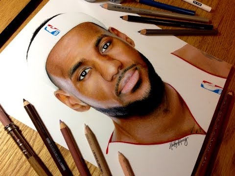
Hand drawn sketch | Models made in CC4 with ZBrush | Textures in Substance Painter | Paint over in Photoshop | Renders, Animation, VFX with AI. Each 5-8 hours spread over a couple days.
As I continue to explore the use of AI tools to enhance my 3D character creation process, I discover they can be incredibly useful during the previsualization phase to see what a character might ultimately look like in production. I selectively use AI to enhance and accelerate my creative process, not to replace it or use it as an end to end solution.
One problem with sRGB is that in a gradient between blue and white, it becomes a bit purple in the middle of the transition. That’s because sRGB really isn’t created to mimic how the eye sees colors; rather, it is based on how CRT monitors work. That means it works with certain frequencies of red, green, and blue, and also the non-linear coding called gamma. It’s a miracle it works as well as it does, but it’s not connected to color perception. When using those tools, you sometimes get surprising results, like purple in the gradient.
There were also attempts to create simple models matching human perception based on XYZ, but as it turned out, it’s not possible to model all color vision that way. Perception of color is incredibly complex and depends, among other things, on whether it is dark or light in the room and the background color it is against. When you look at a photograph, it also depends on what you think the color of the light source is. The dress is a typical example of color vision being very context-dependent. It is almost impossible to model this perfectly.
I based Oklab on two other color spaces, CIECAM16 and IPT. I used the lightness and saturation prediction from CIECAM16, which is a color appearance model, as a target. I actually wanted to use the datasets used to create CIECAM16, but I couldn’t find them.
IPT was designed to have better hue uniformity. In experiments, they asked people to match light and dark colors, saturated and unsaturated colors, which resulted in a dataset for which colors, subjectively, have the same hue. IPT has a few other issues but is the basis for hue in Oklab.
In the Munsell color system, colors are described with three parameters, designed to match the perceived appearance of colors: Hue, Chroma and Value. The parameters are designed to be independent and each have a uniform scale. This results in a color solid with an irregular shape. The parameters are designed to be independent and each have a uniform scale. This results in a color solid with an irregular shape. Modern color spaces and models, such as CIELAB, Cam16 and Björn Ottosson own Oklab, are very similar in their construction.
By far the most used color spaces today for color picking are HSL and HSV, two representations introduced in the classic 1978 paper “Color Spaces for Computer Graphics”. HSL and HSV designed to roughly correlate with perceptual color properties while being very simple and cheap to compute.
Today HSL and HSV are most commonly used together with the sRGB color space.
One of the main advantages of HSL and HSV over the different Lab color spaces is that they map the sRGB gamut to a cylinder. This makes them easy to use since all parameters can be changed independently, without the risk of creating colors outside of the target gamut.
The main drawback on the other hand is that their properties don’t match human perception particularly well.
Reconciling these conflicting goals perfectly isn’t possible, but given that HSV and HSL don’t use anything derived from experiments relating to human perception, creating something that makes a better tradeoff does not seem unreasonable.
With this new lightness estimate, we are ready to look into the construction of Okhsv and Okhsl.
Chroma Key Green, the color of green screens is also known as Chroma Green and is valued at approximately 354C in the Pantone color matching system (PMS).
Chroma Green can be broken down in many different ways. Here is green screen green as other values useful for both physical and digital production:
Green Screen as RGB Color Value: 0, 177, 64
Green Screen as CMYK Color Value: 81, 0, 92, 0
Green Screen as Hex Color Value: #00b140
Green Screen as Websafe Color Value: #009933
Chroma Key Green is reasonably close to an 18% gray reflectance.
Illuminate your green screen with an uniform source with less than 2/3 EV variation.
The level of brightness at any given f-stop should be equivalent to a 90% white card under the same lighting.
A number of problems in computer vision and related fields would be mitigated if camera spectral sensitivities were known. As consumer cameras are not designed for high-precision visual tasks, manufacturers do not disclose spectral sensitivities. Their estimation requires a costly optical setup, which triggered researchers to come up with numerous indirect methods that aim to lower cost and complexity by using color targets. However, the use of color targets gives rise to new complications that make the estimation more difficult, and consequently, there currently exists no simple, low-cost, robust go-to method for spectral sensitivity estimation that non-specialized research labs can adopt. Furthermore, even if not limited by hardware or cost, researchers frequently work with imagery from multiple cameras that they do not have in their possession.
To provide a practical solution to this problem, we propose a framework for spectral sensitivity estimation that not only does not require any hardware (including a color target), but also does not require physical access to the camera itself. Similar to other work, we formulate an optimization problem that minimizes a two-term objective function: a camera-specific term from a system of equations, and a universal term that bounds the solution space.
Different than other work, we utilize publicly available high-quality calibration data to construct both terms. We use the colorimetric mapping matrices provided by the Adobe DNG Converter to formulate the camera-specific system of equations, and constrain the solutions using an autoencoder trained on a database of ground-truth curves. On average, we achieve reconstruction errors as low as those that can arise due to manufacturing imperfections between two copies of the same camera. We provide predicted sensitivities for more than 1,000 cameras that the Adobe DNG Converter currently supports, and discuss which tasks can become trivial when camera responses are available.
This page compares images rendered in Arnold using spectral rendering and different sets of colourspace primaries: Rec.709, Rec.2020, ACES and DCI-P3. The SPD data for the GretagMacbeth Color Checker are the measurements of Noburu Ohta, taken from Mansencal, Mauderer and Parsons (2014) colour-science.org.
The human eye perceives half scene brightness not as the linear 50% of the present energy (linear nature values) but as 18% of the overall brightness. We are biased to perceive more information in the dark and contrast areas. A Macbeth chart helps with calibrating back into a photographic capture into this “human perspective” of the world.
In photography, painting, and other visual arts, middle gray or middle grey is a tone that is perceptually about halfway between black and white on a lightness scale in photography and printing, it is typically defined as 18% reflectance in visible light
Light meters, cameras, and pictures are often calibrated using an 18% gray card[4][5][6] or a color reference card such as a ColorChecker. On the assumption that 18% is similar to the average reflectance of a scene, a grey card can be used to estimate the required exposure of the film.
DISCLAIMER – Links and images on this website may be protected by the respective owners’ copyright. All data submitted by users through this site shall be treated as freely available to share.


![[gamma correction test]](http://www.madore.org/~david/misc/color/gammatest.png "sRGB gamma correction test")


