


COMPOSITION


DESIGN
-
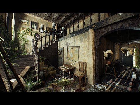
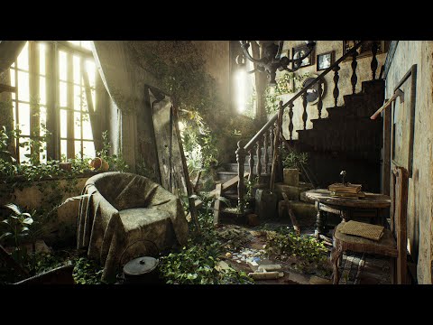
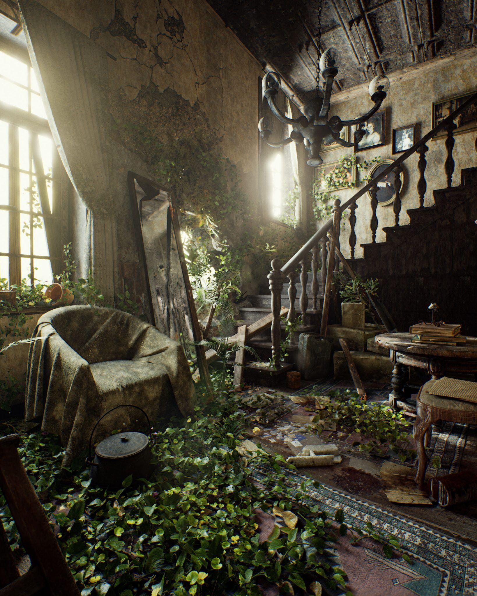
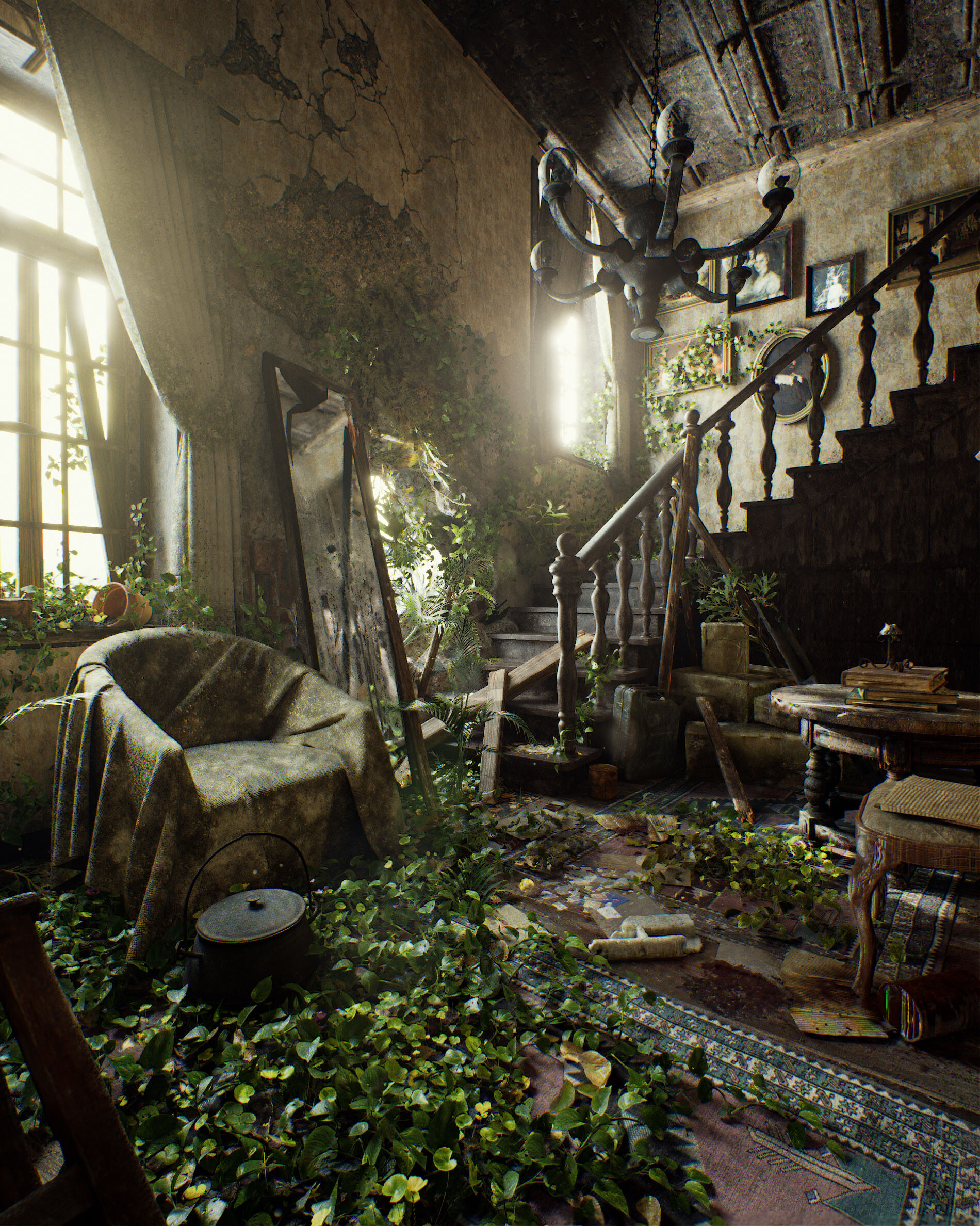
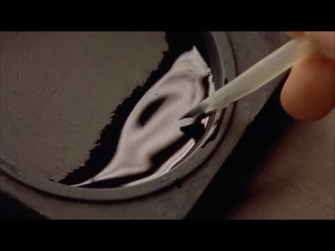
Pasquale Scionti – Production Walkthrough with Virtual Camera and iPad pro 11.5 on Unreal Engine 4.25
Read more: Pasquale Scionti – Production Walkthrough with Virtual Camera and iPad pro 11.5 on Unreal Engine 4.2580.lv/articles/creating-an-old-abandoned-mansion-with-quixel-tools/
www.artstation.com/artwork/Poexyo


COLOR
-
Björn Ottosson – OKHSV and OKHSL – Two new color spaces for color picking
Read more: Björn Ottosson – OKHSV and OKHSL – Two new color spaces for color pickinghttps://bottosson.github.io/misc/colorpicker
https://bottosson.github.io/posts/colorpicker/
https://www.smashingmagazine.com/2024/10/interview-bjorn-ottosson-creator-oklab-color-space/
One problem with sRGB is that in a gradient between blue and white, it becomes a bit purple in the middle of the transition. That’s because sRGB really isn’t created to mimic how the eye sees colors; rather, it is based on how CRT monitors work. That means it works with certain frequencies of red, green, and blue, and also the non-linear coding called gamma. It’s a miracle it works as well as it does, but it’s not connected to color perception. When using those tools, you sometimes get surprising results, like purple in the gradient.

There were also attempts to create simple models matching human perception based on XYZ, but as it turned out, it’s not possible to model all color vision that way. Perception of color is incredibly complex and depends, among other things, on whether it is dark or light in the room and the background color it is against. When you look at a photograph, it also depends on what you think the color of the light source is. The dress is a typical example of color vision being very context-dependent. It is almost impossible to model this perfectly.
I based Oklab on two other color spaces, CIECAM16 and IPT. I used the lightness and saturation prediction from CIECAM16, which is a color appearance model, as a target. I actually wanted to use the datasets used to create CIECAM16, but I couldn’t find them.
IPT was designed to have better hue uniformity. In experiments, they asked people to match light and dark colors, saturated and unsaturated colors, which resulted in a dataset for which colors, subjectively, have the same hue. IPT has a few other issues but is the basis for hue in Oklab.
In the Munsell color system, colors are described with three parameters, designed to match the perceived appearance of colors: Hue, Chroma and Value. The parameters are designed to be independent and each have a uniform scale. This results in a color solid with an irregular shape. The parameters are designed to be independent and each have a uniform scale. This results in a color solid with an irregular shape. Modern color spaces and models, such as CIELAB, Cam16 and Björn Ottosson own Oklab, are very similar in their construction.

By far the most used color spaces today for color picking are HSL and HSV, two representations introduced in the classic 1978 paper “Color Spaces for Computer Graphics”. HSL and HSV designed to roughly correlate with perceptual color properties while being very simple and cheap to compute.
Today HSL and HSV are most commonly used together with the sRGB color space.

One of the main advantages of HSL and HSV over the different Lab color spaces is that they map the sRGB gamut to a cylinder. This makes them easy to use since all parameters can be changed independently, without the risk of creating colors outside of the target gamut.

The main drawback on the other hand is that their properties don’t match human perception particularly well.
Reconciling these conflicting goals perfectly isn’t possible, but given that HSV and HSL don’t use anything derived from experiments relating to human perception, creating something that makes a better tradeoff does not seem unreasonable.
With this new lightness estimate, we are ready to look into the construction of Okhsv and Okhsl.


-
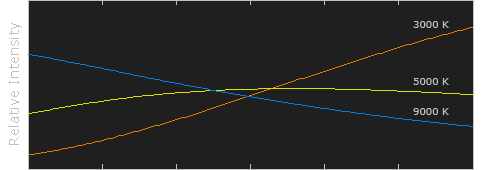
Black Body color aka the Planckian Locus curve for white point eye perception
Read more: Black Body color aka the Planckian Locus curve for white point eye perceptionhttp://en.wikipedia.org/wiki/Black-body_radiation

Black-body radiation is the type of electromagnetic radiation within or surrounding a body in thermodynamic equilibrium with its environment, or emitted by a black body (an opaque and non-reflective body) held at constant, uniform temperature. The radiation has a specific spectrum and intensity that depends only on the temperature of the body.
A black-body at room temperature appears black, as most of the energy it radiates is infra-red and cannot be perceived by the human eye. At higher temperatures, black bodies glow with increasing intensity and colors that range from dull red to blindingly brilliant blue-white as the temperature increases.
The Black Body Ultraviolet Catastrophe Experiment
In photography, color temperature describes the spectrum of light which is radiated from a “blackbody” with that surface temperature. A blackbody is an object which absorbs all incident light — neither reflecting it nor allowing it to pass through.
The Sun closely approximates a black-body radiator. Another rough analogue of blackbody radiation in our day to day experience might be in heating a metal or stone: these are said to become “red hot” when they attain one temperature, and then “white hot” for even higher temperatures. Similarly, black bodies at different temperatures also have varying color temperatures of “white light.”
Despite its name, light which may appear white does not necessarily contain an even distribution of colors across the visible spectrum.
Although planets and stars are neither in thermal equilibrium with their surroundings nor perfect black bodies, black-body radiation is used as a first approximation for the energy they emit. Black holes are near-perfect black bodies, and it is believed that they emit black-body radiation (called Hawking radiation), with a temperature that depends on the mass of the hole.
-
Paul Debevec, Chloe LeGendre, Lukas Lepicovsky – Jointly Optimizing Color Rendition and In-Camera Backgrounds in an RGB Virtual Production Stage
Read more: Paul Debevec, Chloe LeGendre, Lukas Lepicovsky – Jointly Optimizing Color Rendition and In-Camera Backgrounds in an RGB Virtual Production Stagehttps://arxiv.org/pdf/2205.12403.pdf
RGB LEDs vs RGBWP (RGB + lime + phospor converted amber) LEDs
Local copy:
-
Yasuharu YOSHIZAWA – Comparison of sRGB vs ACREScg in Nuke
Read more: Yasuharu YOSHIZAWA – Comparison of sRGB vs ACREScg in NukeAnswering the question that is often asked, “Do I need to use ACEScg to display an sRGB monitor in the end?” (Demonstration shown at an in-house seminar)
Comparison of scanlineRender output with extreme color lights on color charts with sRGB/ACREScg in color – OCIO -working space in NukeDownload the Nuke script:
-
Light and Matter : The 2018 theory of Physically-Based Rendering and Shading by Allegorithmic
Read more: Light and Matter : The 2018 theory of Physically-Based Rendering and Shading by Allegorithmicacademy.substance3d.com/courses/the-pbr-guide-part-1
academy.substance3d.com/courses/the-pbr-guide-part-2

 Local copy:
-
FXGuide – ACES 2.0 with ILM’s Alex Fry
Read more: FXGuide – ACES 2.0 with ILM’s Alex Fry
https://draftdocs.acescentral.com/background/whats-new/
ACES 2.0 is the second major release of the components that make up the ACES system. The most significant change is a new suite of rendering transforms whose design was informed by collected feedback and requests from users of ACES 1. The changes aim to improve the appearance of perceived artifacts and to complete previously unfinished components of the system, resulting in a more complete, robust, and consistent product.
Highlights of the key changes in ACES 2.0 are as follows:
- New output transforms, including:
- A less aggressive tone scale
- More intuitive controls to create custom outputs to non-standard displays
- Robust gamut mapping to improve perceptual uniformity
- Improved performance of the inverse transforms
- Enhanced AMF specification
- An updated specification for ACES Transform IDs
- OpenEXR compression recommendations
- Enhanced tools for generating Input Transforms and recommended procedures for characterizing prosumer cameras
- Look Transform Library
- Expanded documentation
Rendering Transform
The most substantial change in ACES 2.0 is a complete redesign of the rendering transform.
ACES 2.0 was built as a unified system, rather than through piecemeal additions. Different deliverable outputs “match” better and making outputs to display setups other than the provided presets is intended to be user-driven. The rendering transforms are less likely to produce undesirable artifacts “out of the box”, which means less time can be spent fixing problematic images and more time making pictures look the way you want.
Key design goals
- Improve consistency of tone scale and provide an easy to use parameter to allow for outputs between preset dynamic ranges
- Minimize hue skews across exposure range in a region of same hue
- Unify for structural consistency across transform type
- Easy to use parameters to create outputs other than the presets
- Robust gamut mapping to improve harsh clipping artifacts
- Fill extents of output code value cube (where appropriate and expected)
- Invertible – not necessarily reversible, but Output > ACES > Output round-trip should be possible
- Accomplish all of the above while maintaining an acceptable “out-of-the box” rendering
- New output transforms, including:


LIGHTING
-
domeble – Hi-Resolution CGI Backplates and 360° HDRI
Read more: domeble – Hi-Resolution CGI Backplates and 360° HDRIWhen collecting hdri make sure the data supports basic metadata, such as:
- Iso
- Aperture
- Exposure time or shutter time
- Color temperature
- Color space Exposure value (what the sensor receives of the sun intensity in lux)
- 7+ brackets (with 5 or 6 being the perceived balanced exposure)
In image processing, computer graphics, and photography, high dynamic range imaging (HDRI or just HDR) is a set of techniques that allow a greater dynamic range of luminances (a Photometry measure of the luminous intensity per unit area of light travelling in a given direction. It describes the amount of light that passes through or is emitted from a particular area, and falls within a given solid angle) between the lightest and darkest areas of an image than standard digital imaging techniques or photographic methods. This wider dynamic range allows HDR images to represent more accurately the wide range of intensity levels found in real scenes ranging from direct sunlight to faint starlight and to the deepest shadows.
The two main sources of HDR imagery are computer renderings and merging of multiple photographs, which in turn are known as low dynamic range (LDR) or standard dynamic range (SDR) images. Tone Mapping (Look-up) techniques, which reduce overall contrast to facilitate display of HDR images on devices with lower dynamic range, can be applied to produce images with preserved or exaggerated local contrast for artistic effect. Photography
In photography, dynamic range is measured in Exposure Values (in photography, exposure value denotes all combinations of camera shutter speed and relative aperture that give the same exposure. The concept was developed in Germany in the 1950s) differences or stops, between the brightest and darkest parts of the image that show detail. An increase of one EV or one stop is a doubling of the amount of light.
The human response to brightness is well approximated by a Steven’s power law, which over a reasonable range is close to logarithmic, as described by the Weber�Fechner law, which is one reason that logarithmic measures of light intensity are often used as well.
HDR is short for High Dynamic Range. It’s a term used to describe an image which contains a greater exposure range than the “black” to “white” that 8 or 16-bit integer formats (JPEG, TIFF, PNG) can describe. Whereas these Low Dynamic Range images (LDR) can hold perhaps 8 to 10 f-stops of image information, HDR images can describe beyond 30 stops and stored in 32 bit images.

-
HDRI shooting and editing by Xuan Prada and Greg Zaal
Read more: HDRI shooting and editing by Xuan Prada and Greg Zaalwww.xuanprada.com/blog/2014/11/3/hdri-shooting
http://blog.gregzaal.com/2016/03/16/make-your-own-hdri/
http://blog.hdrihaven.com/how-to-create-high-quality-hdri/
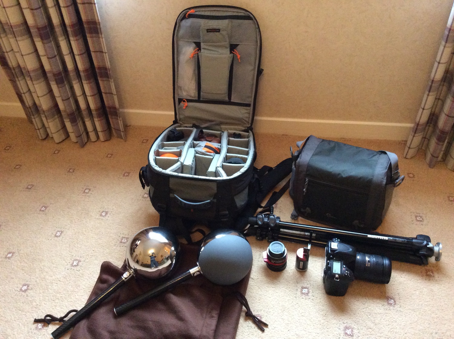
Shooting checklist
- Full coverage of the scene (fish-eye shots)
- Backplates for look-development (including ground or floor)
- Macbeth chart for white balance
- Grey ball for lighting calibration
- Chrome ball for lighting orientation
- Basic scene measurements
- Material samples
- Individual HDR artificial lighting sources if required
Methodology
(more…) -
IES Light Profiles and editing software
Read more: IES Light Profiles and editing softwarehttp://www.derekjenson.com/3d-blog/ies-light-profiles
https://ieslibrary.com/en/browse#ies
https://leomoon.com/store/shaders/ies-lights-pack
https://docs.arnoldrenderer.com/display/a5afmug/ai+photometric+light
IES profiles are useful for creating life-like lighting, as they can represent the physical distribution of light from any light source.
The IES format was created by the Illumination Engineering Society, and most lighting manufacturers provide IES profile for the lights they manufacture.


-
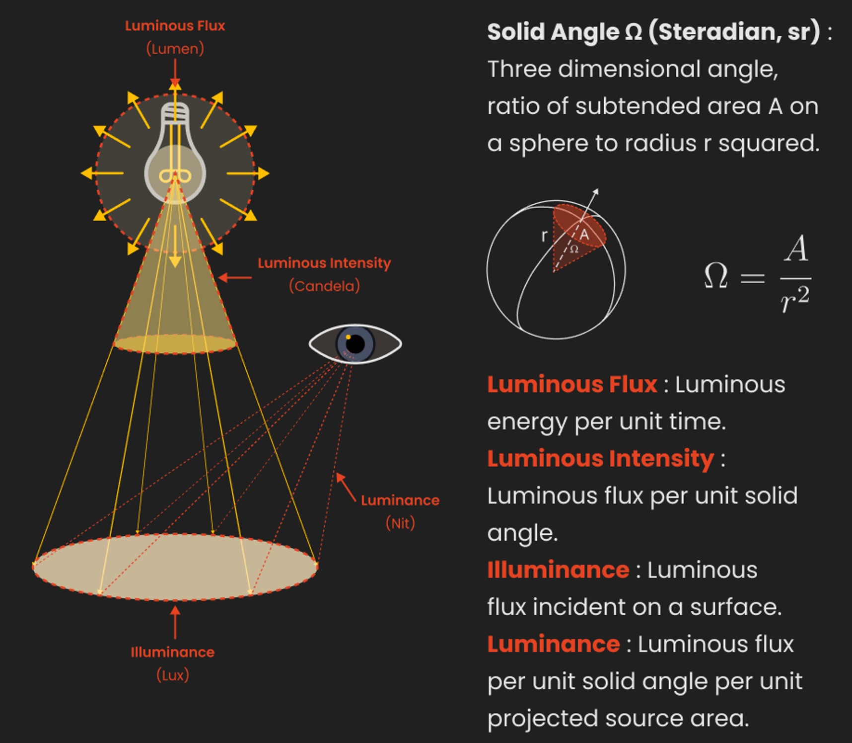
LUX vs LUMEN vs NITS vs CANDELA – What is the difference
Read more: LUX vs LUMEN vs NITS vs CANDELA – What is the differenceMore details here: Lumens vs Candelas (candle) vs Lux vs FootCandle vs Watts vs Irradiance vs Illuminance

https://www.inhouseav.com.au/blog/beginners-guide-nits-lumens-brightness/

Candela
Candela is the basic unit of measure of the entire volume of light intensity from any point in a single direction from a light source. Note the detail: it measures the total volume of light within a certain beam angle and direction.
While the luminance of starlight is around 0.001 cd/m2, that of a sunlit scene is around 100,000 cd/m2, which is a hundred millions times higher. The luminance of the sun itself is approximately 1,000,000,000 cd/m2.NIT
https://en.wikipedia.org/wiki/Candela_per_square_metre
The candela per square metre (symbol: cd/m2) is the unit of luminance in the International System of Units (SI). The unit is based on the candela, the SI unit of luminous intensity, and the square metre, the SI unit of area. The nit (symbol: nt) is a non-SI name also used for this unit (1 nt = 1 cd/m2).[1] The term nit is believed to come from the Latin word nitēre, “to shine”. As a measure of light emitted per unit area, this unit is frequently used to specify the brightness of a display device.
NIT and cd/m2 (candela power) represent the same thing and can be used interchangeably. One nit is equivalent to one candela per square meter, where the candela is the amount of light which has been emitted by a common tallow candle, but NIT is not part of the International System of Units (abbreviated SI, from Systeme International, in French).
It’s easiest to think of a TV as emitting light directly, in much the same way as the Sun does. Nits are simply the measurement of the level of light (luminance) in a given area which the emitting source sends to your eyes or a camera sensor.
The Nit can be considered a unit of visible-light intensity which is often used to specify the brightness level of an LCD.
1 Nit is approximately equal to 3.426 Lumens. To work out a comparable number of Nits to Lumens, you need to multiply the number of Nits by 3.426. If you know the number of Lumens, and wish to know the Nits, simply divide the number of Lumens by 3.426.
Most consumer desktop LCDs have Nits of 200 to 300, the average TV most likely has an output capability of between 100 and 200 Nits, and an HDR TV ranges from 400 to 1,500 Nits.
Virtual Production sets currently sport around 6000 NIT ceiling and 1000 NIT wall panels.The ambient brightness of a sunny day with clear blue skies is between 7000-10,000 nits (between 3000-7000 nits for overcast skies and indirect sunlight).
A bright sunny day can have specular highlights that reach over 100,000 nits. Direct sunlight is around 1,600,000,000 nits.
10,000 nits is also the typical brightness of a fluorescent tube – bright, but not painful to look at.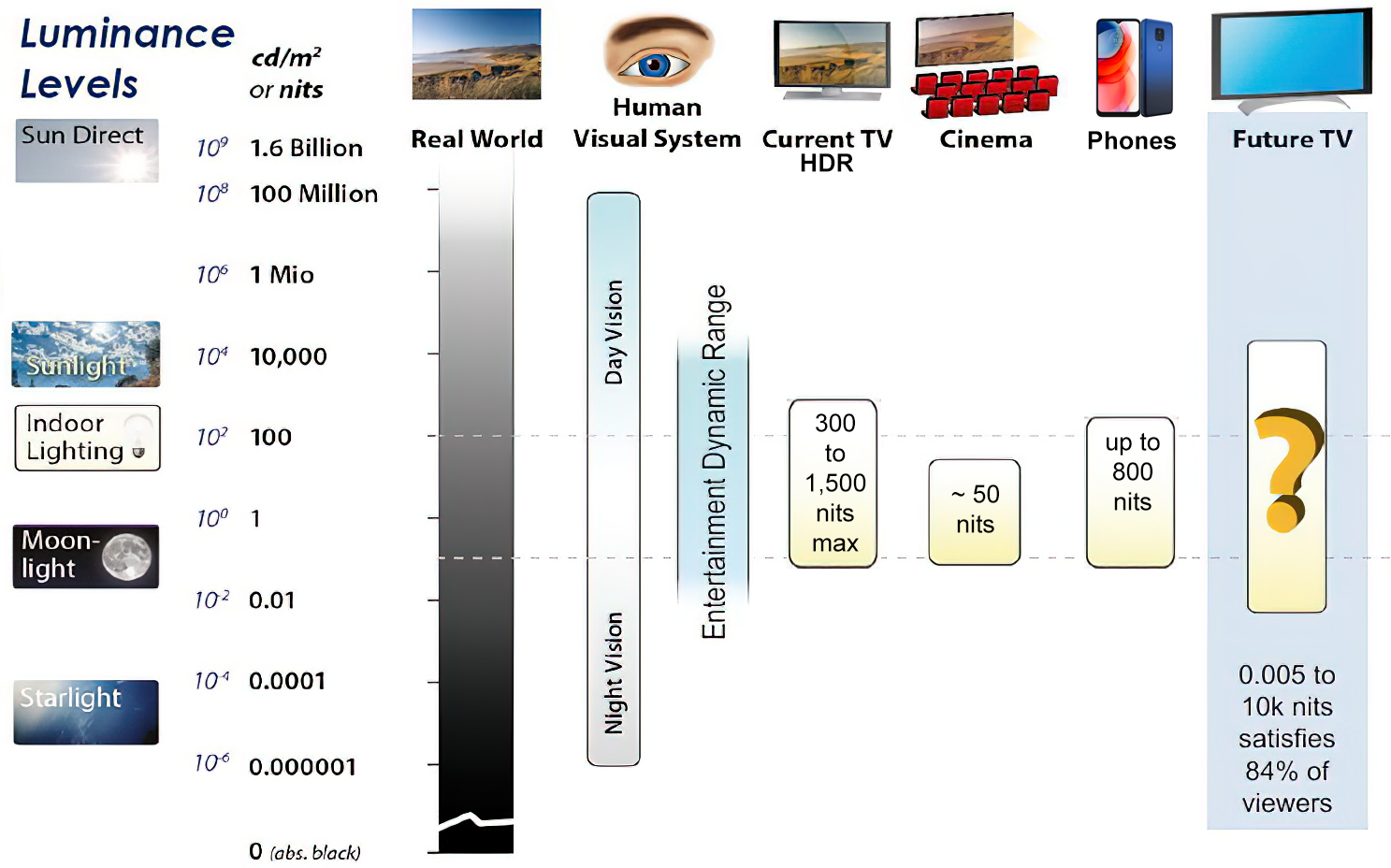
https://www.displaydaily.com/article/display-daily/dolby-vision-vs-hdr10-clarified
Tests showed that a “black level” of 0.005 nits (cd/m²) satisfied the vast majority of viewers. While 0.005 nits is very close to true black, Griffis says Dolby can go down to a black of 0.0001 nits, even though there is no need or ability for displays to get that dark today.
How bright is white? Dolby says the range of 0.005 nits – 10,000 nits satisfied 84% of the viewers in their viewing tests.
The brightest consumer HDR displays today are about 1,500 nits. Professional displays where HDR content is color-graded can achieve up to 4,000 nits peak brightness.High brightness that would be in danger of damaging the eye would be in the neighborhood of 250,000 nits.
Lumens
Lumen is a measure of how much light is emitted (luminance, luminous flux) by an object. It indicates the total potential amount of light from a light source that is visible to the human eye.
Lumen is commonly used in the context of light bulbs or video-projectors as a metric for their brightness power.Lumen is used to describe light output, and about video projectors, it is commonly referred to as ANSI Lumens. Simply put, lumens is how to find out how bright a LED display is. The higher the lumens, the brighter to display!
Technically speaking, a Lumen is the SI unit of luminous flux, which is equal to the amount of light which is emitted per second in a unit solid angle of one steradian from a uniform source of one-candela intensity radiating in all directions.
LUX
Lux (lx) or often Illuminance, is a photometric unit along a given area, which takes in account the sensitivity of human eye to different wavelenghts. It is the measure of light at a specific distance within a specific area at that distance. Often used to measure the incidental sun’s intensity.


COLLECTIONS
| Featured AI
| Design And Composition
| Explore posts
POPULAR SEARCHES
unreal | pipeline | virtual production | free | learn | photoshop | 360 | macro | google | nvidia | resolution | open source | hdri | real-time | photography basics | nuke
FEATURED POSTS
-
3D Gaussian Splatting step by step beginner course
-
Most common ways to smooth 3D prints
-
Key/Fill ratios and scene composition using false colors and Nuke node
-
Eddie Yoon – There’s a big misconception about AI creative
-
What the Boeing 737 MAX’s crashes can teach us about production business – the effects of commoditisation
-
Web vs Printing or digital RGB vs CMYK
-
AnimationXpress.com interviews Daniele Tosti for TheCgCareer.com channel
-
AI Search – Find The Best AI Tools & Apps
Social Links
DISCLAIMER – Links and images on this website may be protected by the respective owners’ copyright. All data submitted by users through this site shall be treated as freely available to share.
