


COMPOSITION
DESIGN
-
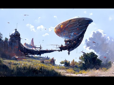
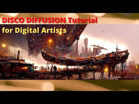
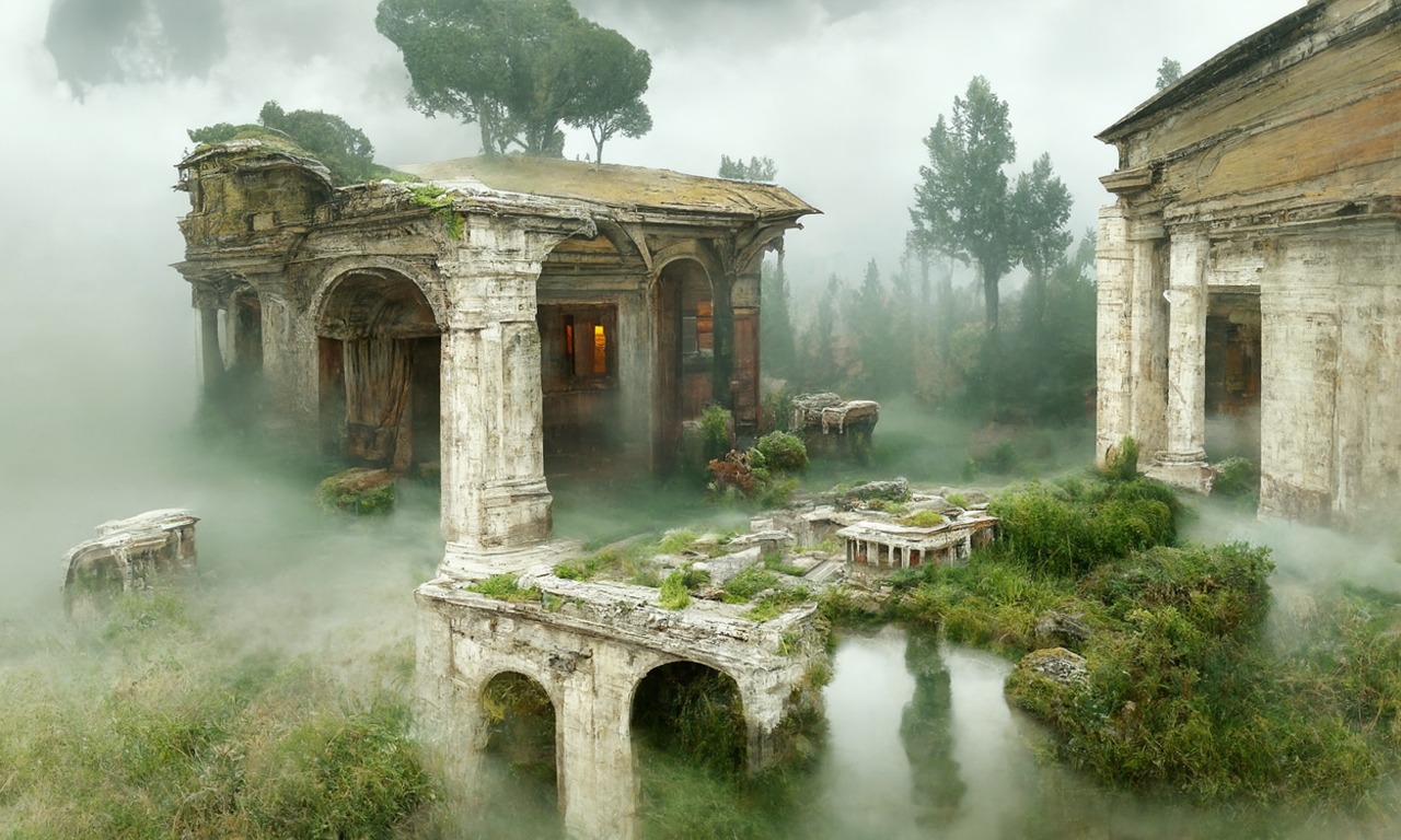
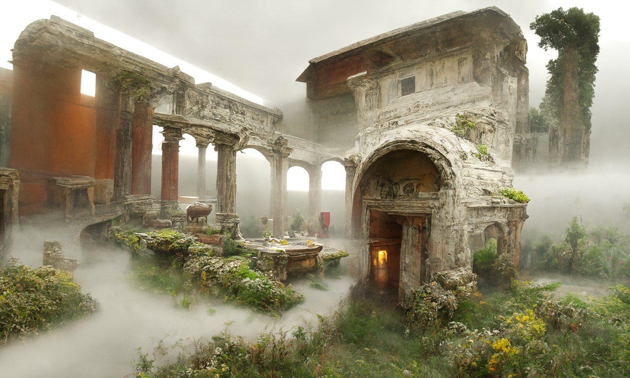
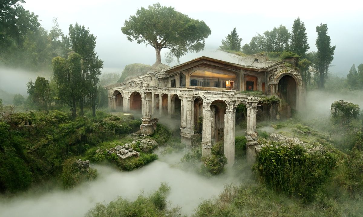
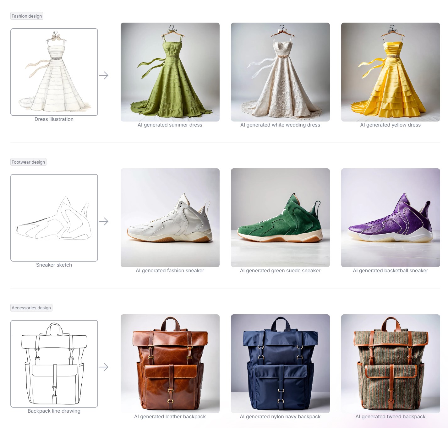
Disco Diffusion V4.1 Google Colab, Dall-E, Starryai – creating images with AI
Read more: Disco Diffusion V4.1 Google Colab, Dall-E, Starryai – creating images with AIDisco Diffusion (DD) is a Google Colab Notebook which leverages an AI Image generating technique called CLIP-Guided Diffusion to allow you to create compelling and beautiful images from just text inputs. Created by Somnai, augmented by Gandamu, and building on the work of RiversHaveWings, nshepperd, and many others.
Phone app: https://www.starryai.com/
docs.google.com/document/d/1l8s7uS2dGqjztYSjPpzlmXLjl5PM3IGkRWI3IiCuK7g
colab.research.google.com/drive/1sHfRn5Y0YKYKi1k-ifUSBFRNJ8_1sa39
Colab, or “Colaboratory”, allows you to write and execute Python in your browser, with
– Zero configuration required
– Access to GPUs free of charge
– Easy sharing
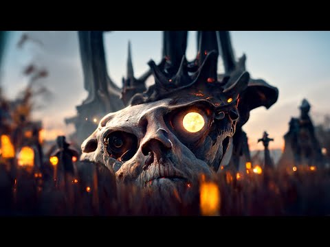

https://80.lv/articles/a-beautiful-roman-villa-made-with-disco-diffusion-5-2/


COLOR
-
A Brief History of Color in Art
Read more: A Brief History of Color in Artwww.artsy.net/article/the-art-genome-project-a-brief-history-of-color-in-art
Of all the pigments that have been banned over the centuries, the color most missed by painters is likely Lead White.
This hue could capture and reflect a gleam of light like no other, though its production was anything but glamorous. The 17th-century Dutch method for manufacturing the pigment involved layering cow and horse manure over lead and vinegar. After three months in a sealed room, these materials would combine to create flakes of pure white. While scientists in the late 19th century identified lead as poisonous, it wasn’t until 1978 that the United States banned the production of lead white paint.

More reading:
www.canva.com/learn/color-meanings/https://www.infogrades.com/history-events-infographics/bizarre-history-of-colors/

-
Colour – MacBeth Chart Checker Detection
Read more: Colour – MacBeth Chart Checker Detectiongithub.com/colour-science/colour-checker-detection
A Python package implementing various colour checker detection algorithms and related utilities.

-
PTGui 13 beta adds control through a Patch Editor
Read more: PTGui 13 beta adds control through a Patch EditorAdditions:
- Patch Editor (PTGui Pro)
- DNG output
- Improved RAW / DNG handling
- JPEG 2000 support
- Performance improvements

-
Light and Matter : The 2018 theory of Physically-Based Rendering and Shading by Allegorithmic
Read more: Light and Matter : The 2018 theory of Physically-Based Rendering and Shading by Allegorithmicacademy.substance3d.com/courses/the-pbr-guide-part-1
academy.substance3d.com/courses/the-pbr-guide-part-2

 Local copy:
-
Yasuharu YOSHIZAWA – Comparison of sRGB vs ACREScg in Nuke
Read more: Yasuharu YOSHIZAWA – Comparison of sRGB vs ACREScg in NukeAnswering the question that is often asked, “Do I need to use ACEScg to display an sRGB monitor in the end?” (Demonstration shown at an in-house seminar)
Comparison of scanlineRender output with extreme color lights on color charts with sRGB/ACREScg in color – OCIO -working space in NukeDownload the Nuke script:


LIGHTING
-
StudioBinder.com – CRI color rendering index
Read more: StudioBinder.com – CRI color rendering indexwww.studiobinder.com/blog/what-is-color-rendering-index
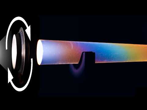
“The Color Rendering Index is a measurement of how faithfully a light source reveals the colors of whatever it illuminates, it describes the ability of a light source to reveal the color of an object, as compared to the color a natural light source would provide. The highest possible CRI is 100. A CRI of 100 generally refers to a perfect black body, like a tungsten light source or the sun. ”


www.pixelsham.com/2021/04/28/types-of-film-lights-and-their-efficiency


COLLECTIONS
| Featured AI
| Design And Composition
| Explore posts
POPULAR SEARCHES
unreal | pipeline | virtual production | free | learn | photoshop | 360 | macro | google | nvidia | resolution | open source | hdri | real-time | photography basics | nuke
FEATURED POSTS
Social Links
DISCLAIMER – Links and images on this website may be protected by the respective owners’ copyright. All data submitted by users through this site shall be treated as freely available to share.
