To measure the contrast ratio you will need a light meter. The process starts with you measuring the main source of light, or the key light.
Get a reading from the brightest area on the face of your subject. Then, measure the area lit by the secondary light, or fill light. To make sense of what you have just measured you have to understand that the information you have just gathered is in F-stops, a measure of light. With each additional F-stop, for example going one stop from f/1.4 to f/2.0, you create a doubling of light. The reverse is also true; moving one stop from f/8.0 to f/5.6 results in a halving of the light.
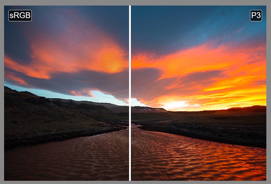
One problem with sRGB is that in a gradient between blue and white, it becomes a bit purple in the middle of the transition. That’s because sRGB really isn’t created to mimic how the eye sees colors; rather, it is based on how CRT monitors work. That means it works with certain frequencies of red, green, and blue, and also the non-linear coding called gamma. It’s a miracle it works as well as it does, but it’s not connected to color perception. When using those tools, you sometimes get surprising results, like purple in the gradient.
There were also attempts to create simple models matching human perception based on XYZ, but as it turned out, it’s not possible to model all color vision that way. Perception of color is incredibly complex and depends, among other things, on whether it is dark or light in the room and the background color it is against. When you look at a photograph, it also depends on what you think the color of the light source is. The dress is a typical example of color vision being very context-dependent. It is almost impossible to model this perfectly.
I based Oklab on two other color spaces, CIECAM16 and IPT. I used the lightness and saturation prediction from CIECAM16, which is a color appearance model, as a target. I actually wanted to use the datasets used to create CIECAM16, but I couldn’t find them.
IPT was designed to have better hue uniformity. In experiments, they asked people to match light and dark colors, saturated and unsaturated colors, which resulted in a dataset for which colors, subjectively, have the same hue. IPT has a few other issues but is the basis for hue in Oklab.
In the Munsell color system, colors are described with three parameters, designed to match the perceived appearance of colors: Hue, Chroma and Value. The parameters are designed to be independent and each have a uniform scale. This results in a color solid with an irregular shape. The parameters are designed to be independent and each have a uniform scale. This results in a color solid with an irregular shape. Modern color spaces and models, such as CIELAB, Cam16 and Björn Ottosson own Oklab, are very similar in their construction.
By far the most used color spaces today for color picking are HSL and HSV, two representations introduced in the classic 1978 paper “Color Spaces for Computer Graphics”. HSL and HSV designed to roughly correlate with perceptual color properties while being very simple and cheap to compute.
Today HSL and HSV are most commonly used together with the sRGB color space.
One of the main advantages of HSL and HSV over the different Lab color spaces is that they map the sRGB gamut to a cylinder. This makes them easy to use since all parameters can be changed independently, without the risk of creating colors outside of the target gamut.
The main drawback on the other hand is that their properties don’t match human perception particularly well.
Reconciling these conflicting goals perfectly isn’t possible, but given that HSV and HSL don’t use anything derived from experiments relating to human perception, creating something that makes a better tradeoff does not seem unreasonable.
With this new lightness estimate, we are ready to look into the construction of Okhsv and Okhsl.
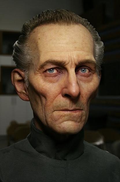
“Memory colors are colors that are universally associated with specific objects, elements or scenes in our environment. They are the colors that we expect to see in specific situations: these colors are based on our expectation of how certain objects should look based on our past experiences and memories.
For instance, we associate specific hues, saturation and brightness values with human skintones and a slight variation can significantly affect the way we perceive a scene.
Similarly, we expect blue skies to have a particular hue, green trees to be a specific shade and so on.
Memory colors live inside of our brains and we often impose them onto what we see. By considering them during the grading process, the resulting image will be more visually appealing and won’t distract the viewer from the intended message of the story. Even a slight deviation from memory colors in a movie can create a sense of discordance, ultimately detracting from the viewer’s experience.”
sRGB: A standard “web”/computer-display RGB color space defined by IEC 61966-2-1. It’s used for most monitors, cameras, printers, and the vast majority of images on the Internet.
Rec. 709: An HD-video color space defined by ITU-R BT.709. It’s the go-to standard for HDTV broadcasts, Blu-ray discs, and professional video pipelines.
Why they exist
sRGB: Ensures consistent colors across different consumer devices (PCs, phones, webcams).
Rec. 709: Ensures consistent colors across video production and playback chains (cameras → editing → broadcast → TV).
What you’ll see
On your desktop or phone, images tagged sRGB will look “right” without extra tweaking.
On an HDTV or video-editing timeline, footage tagged Rec. 709 will display accurate contrast and hue on broadcast-grade monitors.
ACES 2.0 is the second major release of the components that make up the ACES system. The most significant change is a new suite of rendering transforms whose design was informed by collected feedback and requests from users of ACES 1. The changes aim to improve the appearance of perceived artifacts and to complete previously unfinished components of the system, resulting in a more complete, robust, and consistent product.
Highlights of the key changes in ACES 2.0 are as follows:
New output transforms, including:
A less aggressive tone scale
More intuitive controls to create custom outputs to non-standard displays
Robust gamut mapping to improve perceptual uniformity
Improved performance of the inverse transforms
Enhanced AMF specification
An updated specification for ACES Transform IDs
OpenEXR compression recommendations
Enhanced tools for generating Input Transforms and recommended procedures for characterizing prosumer cameras
Look Transform Library
Expanded documentation
Rendering Transform
The most substantial change in ACES 2.0 is a complete redesign of the rendering transform.
ACES 2.0 was built as a unified system, rather than through piecemeal additions. Different deliverable outputs “match” better and making outputs to display setups other than the provided presets is intended to be user-driven. The rendering transforms are less likely to produce undesirable artifacts “out of the box”, which means less time can be spent fixing problematic images and more time making pictures look the way you want.
Key design goals
Improve consistency of tone scale and provide an easy to use parameter to allow for outputs between preset dynamic ranges
Minimize hue skews across exposure range in a region of same hue
Unify for structural consistency across transform type
Easy to use parameters to create outputs other than the presets
Robust gamut mapping to improve harsh clipping artifacts
Fill extents of output code value cube (where appropriate and expected)
Invertible – not necessarily reversible, but Output > ACES > Output round-trip should be possible
Accomplish all of the above while maintaining an acceptable “out-of-the box” rendering
Divesh Naidoo: The video below was made with a live in-camera preview and auto-exposure matching, no camera solve, no HDRI capture and no manual compositing setup. Using the new Simulon phone app.
Note. The Median Cut algorithm is typically used for color quantization, which involves reducing the number of colors in an image while preserving its visual quality. It doesn’t directly provide a way to identify the brightest areas in an image. However, if you’re interested in identifying the brightest areas, you might want to look into other methods like thresholding, histogram analysis, or edge detection, through openCV for example.
Chroma Key Green, the color of green screens is also known as Chroma Green and is valued at approximately 354C in the Pantone color matching system (PMS).
Chroma Green can be broken down in many different ways. Here is green screen green as other values useful for both physical and digital production:
Green Screen as RGB Color Value: 0, 177, 64
Green Screen as CMYK Color Value: 81, 0, 92, 0
Green Screen as Hex Color Value: #00b140
Green Screen as Websafe Color Value: #009933
Chroma Key Green is reasonably close to an 18% gray reflectance.
Illuminate your green screen with an uniform source with less than 2/3 EV variation.
The level of brightness at any given f-stop should be equivalent to a 90% white card under the same lighting.
Black-body radiation is the type of electromagnetic radiation within or surrounding a body in thermodynamic equilibrium with its environment, or emitted by a black body (an opaque and non-reflective body) held at constant, uniform temperature. The radiation has a specific spectrum and intensity that depends only on the temperature of the body.
A black-body at room temperature appears black, as most of the energy it radiates is infra-red and cannot be perceived by the human eye. At higher temperatures, black bodies glow with increasing intensity and colors that range from dull red to blindingly brilliant blue-white as the temperature increases.
DISCLAIMER – Links and images on this website may be protected by the respective owners’ copyright. All data submitted by users through this site shall be treated as freely available to share.


 Local copy:


