One problem with sRGB is that in a gradient between blue and white, it becomes a bit purple in the middle of the transition. That’s because sRGB really isn’t created to mimic how the eye sees colors; rather, it is based on how CRT monitors work. That means it works with certain frequencies of red, green, and blue, and also the non-linear coding called gamma. It’s a miracle it works as well as it does, but it’s not connected to color perception. When using those tools, you sometimes get surprising results, like purple in the gradient.
There were also attempts to create simple models matching human perception based on XYZ, but as it turned out, it’s not possible to model all color vision that way. Perception of color is incredibly complex and depends, among other things, on whether it is dark or light in the room and the background color it is against. When you look at a photograph, it also depends on what you think the color of the light source is. The dress is a typical example of color vision being very context-dependent. It is almost impossible to model this perfectly.
I based Oklab on two other color spaces, CIECAM16 and IPT. I used the lightness and saturation prediction from CIECAM16, which is a color appearance model, as a target. I actually wanted to use the datasets used to create CIECAM16, but I couldn’t find them.
IPT was designed to have better hue uniformity. In experiments, they asked people to match light and dark colors, saturated and unsaturated colors, which resulted in a dataset for which colors, subjectively, have the same hue. IPT has a few other issues but is the basis for hue in Oklab.
In the Munsell color system, colors are described with three parameters, designed to match the perceived appearance of colors: Hue, Chroma and Value. The parameters are designed to be independent and each have a uniform scale. This results in a color solid with an irregular shape. The parameters are designed to be independent and each have a uniform scale. This results in a color solid with an irregular shape. Modern color spaces and models, such as CIELAB, Cam16 and Björn Ottosson own Oklab, are very similar in their construction.
By far the most used color spaces today for color picking are HSL and HSV, two representations introduced in the classic 1978 paper “Color Spaces for Computer Graphics”. HSL and HSV designed to roughly correlate with perceptual color properties while being very simple and cheap to compute.
Today HSL and HSV are most commonly used together with the sRGB color space.
One of the main advantages of HSL and HSV over the different Lab color spaces is that they map the sRGB gamut to a cylinder. This makes them easy to use since all parameters can be changed independently, without the risk of creating colors outside of the target gamut.
The main drawback on the other hand is that their properties don’t match human perception particularly well.
Reconciling these conflicting goals perfectly isn’t possible, but given that HSV and HSL don’t use anything derived from experiments relating to human perception, creating something that makes a better tradeoff does not seem unreasonable.
With this new lightness estimate, we are ready to look into the construction of Okhsv and Okhsl.
In color technology, color depth also known as bit depth, is either the number of bits used to indicate the color of a single pixel, OR the number of bits used for each color component of a single pixel.
When referring to a pixel, the concept can be defined as bits per pixel (bpp).
When referring to a color component, the concept can be defined as bits per component, bits per channel, bits per color (all three abbreviated bpc), and also bits per pixel component, bits per color channel or bits per sample (bps). Modern standards tend to use bits per component, but historical lower-depth systems used bits per pixel more often.
Color depth is only one aspect of color representation, expressing the precision with which the amount of each primary can be expressed; the other aspect is how broad a range of colors can be expressed (the gamut). The definition of both color precision and gamut is accomplished with a color encoding specification which assigns a digital code value to a location in a color space.
The 2011 Best Illusion of the Year uses motion to render color changes invisible, and so reveals a quirk in our visual systems that is new to scientists.
“It is a really beautiful effect, revealing something about how our visual system works that we didn’t know before,” said Daniel Simons, a professor at the University of Illinois, Champaign-Urbana. Simons studies visual cognition, and did not work on this illusion. Before its creation, scientists didn’t know that motion had this effect on perception, Simons said.
A viewer stares at a speck at the center of a ring of colored dots, which continuously change color. When the ring begins to rotate around the speck, the color changes appear to stop. But this is an illusion. For some reason, the motion causes our visual system to ignore the color changes. (You can, however, see the color changes if you follow the rotating circles with your eyes.)
About 576 megapixels for the entire field of view.
Consider a view in front of you that is 90 degrees by 90 degrees, like looking through an open window at a scene. The number of pixels would be:
90 degrees * 60 arc-minutes/degree * 1/0.3 * 90 * 60 * 1/0.3 = 324,000,000 pixels (324 megapixels).
At any one moment, you actually do not perceive that many pixels, but your eye moves around the scene to see all the detail you want. But the human eye really sees a larger field of view, close to 180 degrees. Let’s be conservative and use 120 degrees for the field of view. Then we would see:
Basically, gamma is the relationship between the brightness of a pixel as it appears on the screen, and the numerical value of that pixel. Generally Gamma is just about defining relationships.
Three main types: – Image Gamma encoded in images – Display Gammas encoded in hardware and/or viewing time – System or Viewing Gamma which is the net effect of all gammas when you look back at a final image. In theory this should flatten back to 1.0 gamma.
1 to 100% Stepless Dimming, 1500 Lux Brightness at 3.3′
LCD Info Screen. Powered by an L-series battery, D-Tap, or USB-C
Because the light has a variable color range of 3200 to 9500K, when the light is set to 5500K (daylight balanced) both sets of LEDs are on at full, providing the maximum brightness from this fixture when compared to using the light at 3200 or 9500K.
The LCD screen provides information on the fixture’s output as well as the charge state of the battery. The screen also indicates whether the adjustment knob is controlling brightness or color temperature. To switch from brightness to CCT or CCT to brightness, just apply a short press to the adjustment knob.
The included cold shoe ball joint adapter enables mounting the light to your camera’s accessory shoe via the 1/4″-20 threaded hole on the fixture. In addition, the bottom of the cold shoe foot features a 3/8″-16 threaded hole, and includes a 3/8″-16 to 1/4″-20 reducing bushing.
A way to approximate complex lighting in ultra realistic renders.
All SH lighting techniques involve replacing parts of standard lighting equations with spherical functions that have been projected into frequency space using the spherical harmonics as a basis.
An exposure stop is a unit measurement of Exposure as such it provides a universal linear scale to measure the increase and decrease in light, exposed to the image sensor, due to changes in shutter speed, iso and f-stop.
+-1 stop is a doubling or halving of the amount of light let in when taking a photo
1 EV (exposure value) is just another way to say one stop of exposure change.
Same applies to shutter speed, iso and aperture.
Doubling or halving your shutter speed produces an increase or decrease of 1 stop of exposure.
Doubling or halving your iso speed produces an increase or decrease of 1 stop of exposure.
The trigger phrase is “equirectangular 360 degree panorama”. I would avoid saying “spherical projection” since that tends to result in non-equirectangular spherical images.
Image resolution should always be a 2:1 aspect ratio. 1024 x 512 or 1408 x 704 work quite well and were used in the training data. 2048 x 1024 also works.
I suggest using a weight of 0.5 – 1.5. If you are having issues with the image generating too flat instead of having the necessary spherical distortion, try increasing the weight above 1, though this could negatively impact small details of the image. For Flux guidance, I recommend a value of about 2.5 for realistic scenes.
DISCLAIMER – Links and images on this website may be protected by the respective owners’ copyright. All data submitted by users through this site shall be treated as freely available to share.