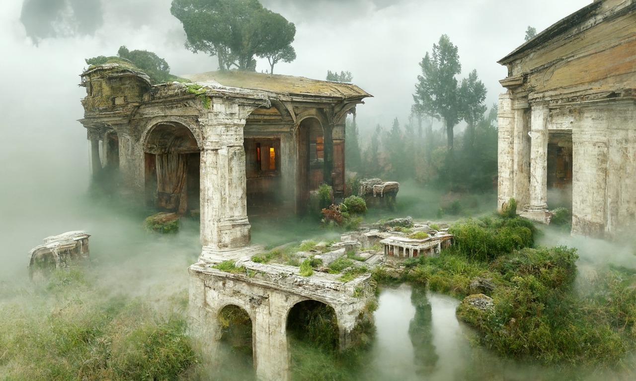
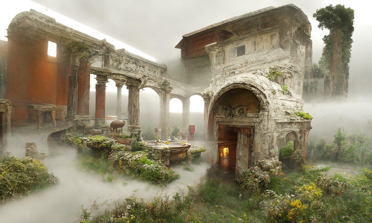
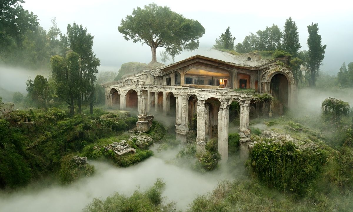
COMPOSITION
-
StudioBinder – Roger Deakins on How to Choose a Camera Lens — Cinematography Composition Techniques
Read more: StudioBinder – Roger Deakins on How to Choose a Camera Lens — Cinematography Composition Techniqueshttps://www.studiobinder.com/blog/camera-lens-buying-guide/
https://www.studiobinder.com/blog/e-books/camera-lenses-explained-volume-1-ebook
DESIGN
-
Arminas Valunas – “Coca-Cola: Wherever you are.”
Read more: Arminas Valunas – “Coca-Cola: Wherever you are.”Arminas created this using Juggernaut Xl model and QR Code Monster SDXL ControlNet.
His pipeline:
Static Images – Forge UI.
Upscaled with Leonardo AI universal upscaler.
Animated with Runway ML and Minimax.
Video upscale – Topaz Video AI.
Composited in Adobe Premiere.
Juggernaut Xl download here:
https://civitai.com/models/133005/juggernaut-xl
QR Code Monster SDXL:
https://civitai.com/models/197247?modelVersionId=221829
COLOR
-
The Forbidden colors – Red-Green & Blue-Yellow: The Stunning Colors You Can’t See
Read more: The Forbidden colors – Red-Green & Blue-Yellow: The Stunning Colors You Can’t Seewww.livescience.com/17948-red-green-blue-yellow-stunning-colors.html

While the human eye has red, green, and blue-sensing cones, those cones are cross-wired in the retina to produce a luminance channel plus a red-green and a blue-yellow channel, and it’s data in that color space (known technically as “LAB”) that goes to the brain. That’s why we can’t perceive a reddish-green or a yellowish-blue, whereas such colors can be represented in the RGB color space used by digital cameras.
https://en.rockcontent.com/blog/the-use-of-yellow-in-data-design
The back of the retina is covered in light-sensitive neurons known as cone cells and rod cells. There are three types of cone cells, each sensitive to different ranges of light. These ranges overlap, but for convenience the cones are referred to as blue (short-wavelength), green (medium-wavelength), and red (long-wavelength). The rod cells are primarily used in low-light situations, so we’ll ignore those for now.
When light enters the eye and hits the cone cells, the cones get excited and send signals to the brain through the visual cortex. Different wavelengths of light excite different combinations of cones to varying levels, which generates our perception of color. You can see that the red cones are most sensitive to light, and the blue cones are least sensitive. The sensitivity of green and red cones overlaps for most of the visible spectrum.

Here’s how your brain takes the signals of light intensity from the cones and turns it into color information. To see red or green, your brain finds the difference between the levels of excitement in your red and green cones. This is the red-green channel.
To get “brightness,” your brain combines the excitement of your red and green cones. This creates the luminance, or black-white, channel. To see yellow or blue, your brain then finds the difference between this luminance signal and the excitement of your blue cones. This is the yellow-blue channel.
From the calculations made in the brain along those three channels, we get four basic colors: blue, green, yellow, and red. Seeing blue is what you experience when low-wavelength light excites the blue cones more than the green and red.
Seeing green happens when light excites the green cones more than the red cones. Seeing red happens when only the red cones are excited by high-wavelength light.
Here’s where it gets interesting. Seeing yellow is what happens when BOTH the green AND red cones are highly excited near their peak sensitivity. This is the biggest collective excitement that your cones ever have, aside from seeing pure white.
Notice that yellow occurs at peak intensity in the graph to the right. Further, the lens and cornea of the eye happen to block shorter wavelengths, reducing sensitivity to blue and violet light.
-
Tim Kang – calibrated white light values in sRGB color space
Read more: Tim Kang – calibrated white light values in sRGB color space8bit sRGB encoded
2000K 255 139 22
2700K 255 172 89
3000K 255 184 109
3200K 255 190 122
4000K 255 211 165
4300K 255 219 178
D50 255 235 205
D55 255 243 224
D5600 255 244 227
D6000 255 249 240
D65 255 255 255
D10000 202 221 255
D20000 166 196 2558bit Rec709 Gamma 2.4
2000K 255 145 34
2700K 255 177 97
3000K 255 187 117
3200K 255 193 129
4000K 255 214 170
4300K 255 221 182
D50 255 236 208
D55 255 243 226
D5600 255 245 229
D6000 255 250 241
D65 255 255 255
D10000 204 222 255
D20000 170 199 2558bit Display P3 encoded
2000K 255 154 63
2700K 255 185 109
3000K 255 195 127
3200K 255 201 138
4000K 255 219 176
4300K 255 225 187
D50 255 239 212
D55 255 245 228
D5600 255 246 231
D6000 255 251 242
D65 255 255 255
D10000 208 223 255
D20000 175 199 25510bit Rec2020 PQ (100 nits)
2000K 520 435 273
2700K 520 466 358
3000K 520 475 384
3200K 520 480 399
4000K 520 495 446
4300K 520 500 458
D50 520 510 482
D55 520 514 497
D5600 520 514 500
D6000 520 517 509
D65 520 520 520
D10000 479 489 520
D20000 448 464 520 -
FXGuide – ACES 2.0 with ILM’s Alex Fry
Read more: FXGuide – ACES 2.0 with ILM’s Alex Fryhttps://draftdocs.acescentral.com/background/whats-new/
ACES 2.0 is the second major release of the components that make up the ACES system. The most significant change is a new suite of rendering transforms whose design was informed by collected feedback and requests from users of ACES 1. The changes aim to improve the appearance of perceived artifacts and to complete previously unfinished components of the system, resulting in a more complete, robust, and consistent product.
Highlights of the key changes in ACES 2.0 are as follows:
- New output transforms, including:
- A less aggressive tone scale
- More intuitive controls to create custom outputs to non-standard displays
- Robust gamut mapping to improve perceptual uniformity
- Improved performance of the inverse transforms
- Enhanced AMF specification
- An updated specification for ACES Transform IDs
- OpenEXR compression recommendations
- Enhanced tools for generating Input Transforms and recommended procedures for characterizing prosumer cameras
- Look Transform Library
- Expanded documentation
Rendering Transform
The most substantial change in ACES 2.0 is a complete redesign of the rendering transform.
ACES 2.0 was built as a unified system, rather than through piecemeal additions. Different deliverable outputs “match” better and making outputs to display setups other than the provided presets is intended to be user-driven. The rendering transforms are less likely to produce undesirable artifacts “out of the box”, which means less time can be spent fixing problematic images and more time making pictures look the way you want.
Key design goals
- Improve consistency of tone scale and provide an easy to use parameter to allow for outputs between preset dynamic ranges
- Minimize hue skews across exposure range in a region of same hue
- Unify for structural consistency across transform type
- Easy to use parameters to create outputs other than the presets
- Robust gamut mapping to improve harsh clipping artifacts
- Fill extents of output code value cube (where appropriate and expected)
- Invertible – not necessarily reversible, but Output > ACES > Output round-trip should be possible
- Accomplish all of the above while maintaining an acceptable “out-of-the box” rendering
- New output transforms, including:
-
Anders Langlands – Render Color Spaces
Read more: Anders Langlands – Render Color Spaceshttps://www.colour-science.org/anders-langlands/
This page compares images rendered in Arnold using spectral rendering and different sets of colourspace primaries: Rec.709, Rec.2020, ACES and DCI-P3. The SPD data for the GretagMacbeth Color Checker are the measurements of Noburu Ohta, taken from Mansencal, Mauderer and Parsons (2014) colour-science.org.
-
Weta Digital – Manuka Raytracer and Gazebo GPU renderers – pipeline
Read more: Weta Digital – Manuka Raytracer and Gazebo GPU renderers – pipelinehttps://jo.dreggn.org/home/2018_manuka.pdf
http://www.fxguide.com/featured/manuka-weta-digitals-new-renderer/

The Manuka rendering architecture has been designed in the spirit of the classic reyes rendering architecture. In its core, reyes is based on stochastic rasterisation of micropolygons, facilitating depth of field, motion blur, high geometric complexity,and programmable shading.
This is commonly achieved with Monte Carlo path tracing, using a paradigm often called shade-on-hit, in which the renderer alternates tracing rays with running shaders on the various ray hits. The shaders take the role of generating the inputs of the local material structure which is then used bypath sampling logic to evaluate contributions and to inform what further rays to cast through the scene.
Over the years, however, the expectations have risen substantially when it comes to image quality. Computing pictures which are indistinguishable from real footage requires accurate simulation of light transport, which is most often performed using some variant of Monte Carlo path tracing. Unfortunately this paradigm requires random memory accesses to the whole scene and does not lend itself well to a rasterisation approach at all.
Manuka is both a uni-directional and bidirectional path tracer and encompasses multiple importance sampling (MIS). Interestingly, and importantly for production character skin work, it is the first major production renderer to incorporate spectral MIS in the form of a new ‘Hero Spectral Sampling’ technique, which was recently published at Eurographics Symposium on Rendering 2014.
Manuka propose a shade-before-hit paradigm in-stead and minimise I/O strain (and some memory costs) on the system, leveraging locality of reference by running pattern generation shaders before we execute light transport simulation by path sampling, “compressing” any bvh structure as needed, and as such also limiting duplication of source data.
The difference with reyes is that instead of baking colors into the geometry like in Reyes, manuka bakes surface closures. This means that light transport is still calculated with path tracing, but all texture lookups etc. are done up-front and baked into the geometry.The main drawback with this method is that geometry has to be tessellated to its highest, stable topology before shading can be evaluated properly. As such, the high cost to first pixel. Even a basic 4 vertices square becomes a much more complex model with this approach.

Manuka use the RenderMan Shading Language (rsl) for programmable shading [Pixar Animation Studios 2015], but we do not invoke rsl shaders when intersecting a ray with a surface (often called shade-on-hit). Instead, we pre-tessellate and pre-shade all the input geometry in the front end of the renderer.
This way, we can efficiently order shading computations to sup-port near-optimal texture locality, vectorisation, and parallelism. This system avoids repeated evaluation of shaders at the same surface point, and presents a minimal amount of memory to be accessed during light transport time. An added benefit is that the acceleration structure for ray tracing (abounding volume hierarchy, bvh) is built once on the final tessellated geometry, which allows us to ray trace more efficiently than multi-level bvhs and avoids costly caching of on-demand tessellated micropolygons and the associated scheduling issues.For the shading reasons above, in terms of AOVs, the studio approach is to succeed at combining complex shading with ray paths in the render rather than pass a multi-pass render to compositing.
For the Spectral Rendering component. The light transport stage is fully spectral, using a continuously sampled wavelength which is traced with each path and used to apply the spectral camera sensitivity of the sensor. This allows for faithfully support any degree of observer metamerism as the camera footage they are intended to match as well as complex materials which require wavelength dependent phenomena such as diffraction, dispersion, interference, iridescence, or chromatic extinction and Rayleigh scattering in participating media.
As opposed to the original reyes paper, we use bilinear interpolation of these bsdf inputs later when evaluating bsdfs per pathv ertex during light transport4. This improves temporal stability of geometry which moves very slowly with respect to the pixel raster
In terms of the pipeline, everything rendered at Weta was already completely interwoven with their deep data pipeline. Manuka very much was written with deep data in mind. Here, Manuka not so much extends the deep capabilities, rather it fully matches the already extremely complex and powerful setup Weta Digital already enjoy with RenderMan. For example, an ape in a scene can be selected, its ID is available and a NUKE artist can then paint in 3D say a hand and part of the way up the neutral posed ape.
We called our system Manuka, as a respectful nod to reyes: we had heard a story froma former ILM employee about how reyes got its name from how fond the early Pixar people were of their lunches at Point Reyes, and decided to name our system after our surrounding natural environment, too. Manuka is a kind of tea tree very common in New Zealand which has very many very small leaves, in analogy to micropolygons ina tree structure for ray tracing. It also happens to be the case that Weta Digital’s main site is on Manuka Street.

-
THOMAS MANSENCAL – The Apparent Simplicity of RGB Rendering
Read more: THOMAS MANSENCAL – The Apparent Simplicity of RGB Renderinghttps://thomasmansencal.substack.com/p/the-apparent-simplicity-of-rgb-rendering
The primary goal of physically-based rendering (PBR) is to create a simulation that accurately reproduces the imaging process of electro-magnetic spectrum radiation incident to an observer. This simulation should be indistinguishable from reality for a similar observer.
Because a camera is not sensitive to incident light the same way than a human observer, the images it captures are transformed to be colorimetric. A project might require infrared imaging simulation, a portion of the electro-magnetic spectrum that is invisible to us. Radically different observers might image the same scene but the act of observing does not change the intrinsic properties of the objects being imaged. Consequently, the physical modelling of the virtual scene should be independent of the observer.
LIGHTING
-
Composition and The Expressive Nature Of Light
Read more: Composition and The Expressive Nature Of Lighthttp://www.huffingtonpost.com/bill-danskin/post_12457_b_10777222.html
George Sand once said “ The artist vocation is to send light into the human heart.”
-
Gamma correction
Read more: Gamma correction
http://www.normankoren.com/makingfineprints1A.html#Gammabox
https://en.wikipedia.org/wiki/Gamma_correction
http://www.photoscientia.co.uk/Gamma.htm
https://www.w3.org/Graphics/Color/sRGB.html
http://www.eizoglobal.com/library/basics/lcd_display_gamma/index.html
https://forum.reallusion.com/PrintTopic308094.aspx
Basically, gamma is the relationship between the brightness of a pixel as it appears on the screen, and the numerical value of that pixel. Generally Gamma is just about defining relationships.
Three main types:
– Image Gamma encoded in images
– Display Gammas encoded in hardware and/or viewing time
– System or Viewing Gamma which is the net effect of all gammas when you look back at a final image. In theory this should flatten back to 1.0 gamma.
(more…) -
Capturing the world in HDR for real time projects – Call of Duty: Advanced Warfare
Read more: Capturing the world in HDR for real time projects – Call of Duty: Advanced WarfareReal-World Measurements for Call of Duty: Advanced Warfare
www.activision.com/cdn/research/Real_World_Measurements_for_Call_of_Duty_Advanced_Warfare.pdf
Local version
Real_World_Measurements_for_Call_of_Duty_Advanced_Warfare.pdf
-
Photography basics: Why Use a (MacBeth) Color Chart?
Read more: Photography basics: Why Use a (MacBeth) Color Chart?Start here: https://www.pixelsham.com/2013/05/09/gretagmacbeth-color-checker-numeric-values/
https://www.studiobinder.com/blog/what-is-a-color-checker-tool/
In LightRoom
in Final Cut
in Nuke
Note: In Foundry’s Nuke, the software will map 18% gray to whatever your center f/stop is set to in the viewer settings (f/8 by default… change that to EV by following the instructions below).
You can experiment with this by attaching an Exposure node to a Constant set to 0.18, setting your viewer read-out to Spotmeter, and adjusting the stops in the node up and down. You will see that a full stop up or down will give you the respective next value on the aperture scale (f8, f11, f16 etc.).One stop doubles or halves the amount or light that hits the filmback/ccd, so everything works in powers of 2.
So starting with 0.18 in your constant, you will see that raising it by a stop will give you .36 as a floating point number (in linear space), while your f/stop will be f/11 and so on.If you set your center stop to 0 (see below) you will get a relative readout in EVs, where EV 0 again equals 18% constant gray.
In other words. Setting the center f-stop to 0 means that in a neutral plate, the middle gray in the macbeth chart will equal to exposure value 0. EV 0 corresponds to an exposure time of 1 sec and an aperture of f/1.0.
This will set the sun usually around EV12-17 and the sky EV1-4 , depending on cloud coverage.
To switch Foundry’s Nuke’s SpotMeter to return the EV of an image, click on the main viewport, and then press s, this opens the viewer’s properties. Now set the center f-stop to 0 in there. And the SpotMeter in the viewport will change from aperture and fstops to EV.
-
RawTherapee – a free, open source, cross-platform raw image and HDRi processing program
Read more: RawTherapee – a free, open source, cross-platform raw image and HDRi processing program5.10 of this tool includes excellent tools to clean up cr2 and cr3 used on set to support HDRI processing.
Converting raw to AcesCG 32 bit tiffs with metadata.
COLLECTIONS
| Featured AI
| Design And Composition
| Explore posts
POPULAR SEARCHES
unreal | pipeline | virtual production | free | learn | photoshop | 360 | macro | google | nvidia | resolution | open source | hdri | real-time | photography basics | nuke
FEATURED POSTS
-
Canva bought Affinity – Now Affinity Photo and Affinity Designer are… GONE?!
-
Godot Cheat Sheets
-
Blender VideoDepthAI – Turn any video into 3D Animated Scenes
-
Black Body color aka the Planckian Locus curve for white point eye perception
-
Tencent Hunyuan3D 2.1 goes Open Source and adds MV (Multi-view) and MV Mini
-
Jesse Zumstein – Jobs in games
-
Alejandro Villabón and Rafał Kaniewski – Recover Highlights With 8-Bit to High Dynamic Range Half Float Copycat – Nuke
-
copypastecharacter.com – alphabets, special characters, alt codes and symbols library
Social Links
DISCLAIMER – Links and images on this website may be protected by the respective owners’ copyright. All data submitted by users through this site shall be treated as freely available to share.


