


COMPOSITION
-
SlowMoVideo – How to make a slow motion shot with the open source program
Read more: SlowMoVideo – How to make a slow motion shot with the open source programhttp://slowmovideo.granjow.net/
slowmoVideo is an OpenSource program that creates slow-motion videos from your footage.
Slow motion cinematography is the result of playing back frames for a longer duration than they were exposed. For example, if you expose 240 frames of film in one second, then play them back at 24 fps, the resulting movie is 10 times longer (slower) than the original filmed event….
Film cameras are relatively simple mechanical devices that allow you to crank up the speed to whatever rate the shutter and pull-down mechanism allow. Some film cameras can operate at 2,500 fps or higher (although film shot in these cameras often needs some readjustment in postproduction). Video, on the other hand, is always captured, recorded, and played back at a fixed rate, with a current limit around 60fps. This makes extreme slow motion effects harder to achieve (and less elegant) on video, because slowing down the video results in each frame held still on the screen for a long time, whereas with high-frame-rate film there are plenty of frames to fill the longer durations of time. On video, the slow motion effect is more like a slide show than smooth, continuous motion.
One obvious solution is to shoot film at high speed, then transfer it to video (a case where film still has a clear advantage, sorry George). Another possibility is to cross dissolve or blur from one frame to the next. This adds a smooth transition from one still frame to the next. The blur reduces the sharpness of the image, and compared to slowing down images shot at a high frame rate, this is somewhat of a cheat. However, there isn’t much you can do about it until video can be recorded at much higher rates. Of course, many film cameras can’t shoot at high frame rates either, so the whole super-slow-motion endeavor is somewhat specialized no matter what medium you are using. (There are some high speed digital cameras available now that allow you to capture lots of digital frames directly to your computer, so technology is starting to catch up with film. However, this feature isn’t going to appear in consumer camcorders any time soon.)
-
7 Commandments of Film Editing and composition
Read more: 7 Commandments of Film Editing and composition
1. Watch every frame of raw footage twice. On the second time, take notes. If you don’t do this and try to start developing a scene premature, then it’s a big disservice to yourself and to the director, actors and production crew.
2. Nurture the relationships with the director. You are the secondary person in the relationship. Be calm and continually offer solutions. Get the main intention of the film as soon as possible from the director.
3. Organize your media so that you can find any shot instantly.
4. Factor in extra time for renders, exports, errors and crashes.
5. Attempt edits and ideas that shouldn’t work. It just might work. Until you do it and watch it, you won’t know. Don’t rule out ideas just because they don’t make sense in your mind.
6. Spend more time on your audio. It’s the glue of your edit. AUDIO SAVES EVERYTHING. Create fluid and seamless audio under your video.
7. Make cuts for the scene, but always in context for the whole film. Have a macro and a micro view at all times.
-
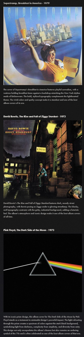
Composition – cinematography Cheat Sheet
Read more: Composition – cinematography Cheat Sheet
Where is our eye attracted first? Why?
Size. Focus. Lighting. Color.
Size. Mr. White (Harvey Keitel) on the right.
Focus. He’s one of the two objects in focus.
Lighting. Mr. White is large and in focus and Mr. Pink (Steve Buscemi) is highlighted by
a shaft of light.
Color. Both are black and white but the read on Mr. White’s shirt now really stands out.
(more…)
What type of lighting? -
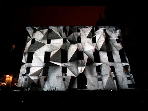
Composition and The Expressive Nature Of Light
Read more: Composition and The Expressive Nature Of Lighthttp://www.huffingtonpost.com/bill-danskin/post_12457_b_10777222.html
George Sand once said “ The artist vocation is to send light into the human heart.”


DESIGN


COLOR
-
Björn Ottosson – How software gets color wrong
Read more: Björn Ottosson – How software gets color wronghttps://bottosson.github.io/posts/colorwrong/
Most software around us today are decent at accurately displaying colors. Processing of colors is another story unfortunately, and is often done badly.
To understand what the problem is, let’s start with an example of three ways of blending green and magenta:
- Perceptual blend – A smooth transition using a model designed to mimic human perception of color. The blending is done so that the perceived brightness and color varies smoothly and evenly.
- Linear blend – A model for blending color based on how light behaves physically. This type of blending can occur in many ways naturally, for example when colors are blended together by focus blur in a camera or when viewing a pattern of two colors at a distance.
- sRGB blend – This is how colors would normally be blended in computer software, using sRGB to represent the colors.

Let’s look at some more examples of blending of colors, to see how these problems surface more practically. The examples use strong colors since then the differences are more pronounced. This is using the same three ways of blending colors as the first example.

Instead of making it as easy as possible to work with color, most software make it unnecessarily hard, by doing image processing with representations not designed for it. Approximating the physical behavior of light with linear RGB models is one easy thing to do, but more work is needed to create image representations tailored for image processing and human perception.
Also see:


LIGHTING
-
Polarised vs unpolarized filtering
Read more: Polarised vs unpolarized filteringA light wave that is vibrating in more than one plane is referred to as unpolarized light. …
Polarized light waves are light waves in which the vibrations occur in a single plane. The process of transforming unpolarized light into polarized light is known as polarization.

en.wikipedia.org/wiki/Polarizing_filter_(photography)
The most common use of polarized technology is to reduce lighting complexity on the subject.
(more…)
Details such as glare and hard edges are not removed, but greatly reduced. -
StudioBinder.com – CRI color rendering index
Read more: StudioBinder.com – CRI color rendering indexwww.studiobinder.com/blog/what-is-color-rendering-index
“The Color Rendering Index is a measurement of how faithfully a light source reveals the colors of whatever it illuminates, it describes the ability of a light source to reveal the color of an object, as compared to the color a natural light source would provide. The highest possible CRI is 100. A CRI of 100 generally refers to a perfect black body, like a tungsten light source or the sun. ”


www.pixelsham.com/2021/04/28/types-of-film-lights-and-their-efficiency
-
Is a MacBeth Colour Rendition Chart the Safest Way to Calibrate a Camera?
Read more: Is a MacBeth Colour Rendition Chart the Safest Way to Calibrate a Camera?www.colour-science.org/posts/the-colorchecker-considered-mostly-harmless/
Video Player00:0000:00“Unless you have all the relevant spectral measurements, a colour rendition chart should not be used to perform colour-correction of camera imagery but only for white balancing and relative exposure adjustments.”
“Using a colour rendition chart for colour-correction might dramatically increase error if the scene light source spectrum is different from the illuminant used to compute the colour rendition chart’s reference values.”
“other factors make using a colour rendition chart unsuitable for camera calibration:
– Uncontrolled geometry of the colour rendition chart with the incident illumination and the camera.
– Unknown sample reflectances and ageing as the colour of the samples vary with time.
– Low samples count.
– Camera noise and flare.
– Etc…“Those issues are well understood in the VFX industry, and when receiving plates, we almost exclusively use colour rendition charts to white balance and perform relative exposure adjustments, i.e. plate neutralisation.”
-
Rec-2020 – TVs new color gamut standard used by Dolby Vision?
Read more: Rec-2020 – TVs new color gamut standard used by Dolby Vision?https://www.hdrsoft.com/resources/dri.html#bit-depth

The dynamic range is a ratio between the maximum and minimum values of a physical measurement. Its definition depends on what the dynamic range refers to.
For a scene: Dynamic range is the ratio between the brightest and darkest parts of the scene.
For a camera: Dynamic range is the ratio of saturation to noise. More specifically, the ratio of the intensity that just saturates the camera to the intensity that just lifts the camera response one standard deviation above camera noise.
For a display: Dynamic range is the ratio between the maximum and minimum intensities emitted from the screen.
The Dynamic Range of real-world scenes can be quite high — ratios of 100,000:1 are common in the natural world. An HDR (High Dynamic Range) image stores pixel values that span the whole tonal range of real-world scenes. Therefore, an HDR image is encoded in a format that allows the largest range of values, e.g. floating-point values stored with 32 bits per color channel. Another characteristics of an HDR image is that it stores linear values. This means that the value of a pixel from an HDR image is proportional to the amount of light measured by the camera.
For TVs HDR is great, but it’s not the only new TV feature worth discussing.
(more…)


COLLECTIONS
| Featured AI
| Design And Composition
| Explore posts
POPULAR SEARCHES
unreal | pipeline | virtual production | free | learn | photoshop | 360 | macro | google | nvidia | resolution | open source | hdri | real-time | photography basics | nuke
FEATURED POSTS
-
Glossary of Lighting Terms – cheat sheet
-
How do LLMs like ChatGPT (Generative Pre-Trained Transformer) work? Explained by Deep-Fake Ryan Gosling
-
Matt Hallett – WAN 2.1 VACE Total Video Control in ComfyUI
-
Kling 1.6 and competitors – advanced tests and comparisons
-
Photography basics: Solid Angle measures
-
Python and TCL: Tips and Tricks for Foundry Nuke
-
Decart AI Mirage – The first ever World Transformation Model – turning any video, game, or camera feed into a new digital world, in real time
-
Animation/VFX/Game Industry JOB POSTINGS by Chris Mayne
Social Links
DISCLAIMER – Links and images on this website may be protected by the respective owners’ copyright. All data submitted by users through this site shall be treated as freely available to share.
