


COMPOSITION
-
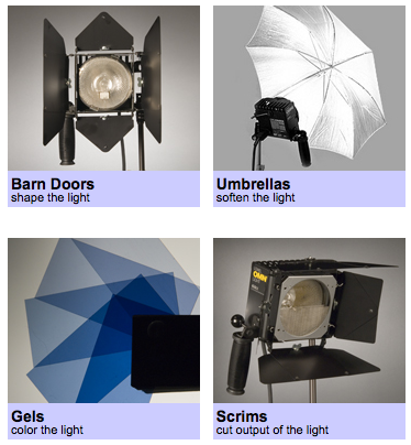
Composition – These are the basic lighting techniques you need to know for photography and film
Read more: Composition – These are the basic lighting techniques you need to know for photography and film
http://www.diyphotography.net/basic-lighting-techniques-need-know-photography-film/
Amongst the basic techniques, there’s…
1- Side lighting – Literally how it sounds, lighting a subject from the side when they’re faced toward you
2- Rembrandt lighting – Here the light is at around 45 degrees over from the front of the subject, raised and pointing down at 45 degrees
3- Back lighting – Again, how it sounds, lighting a subject from behind. This can help to add drama with silouettes
4- Rim lighting – This produces a light glowing outline around your subject
5- Key light – The main light source, and it’s not necessarily always the brightest light source
6- Fill light – This is used to fill in the shadows and provide detail that would otherwise be blackness
7- Cross lighting – Using two lights placed opposite from each other to light two subjects
-
SlowMoVideo – How to make a slow motion shot with the open source program
Read more: SlowMoVideo – How to make a slow motion shot with the open source programhttp://slowmovideo.granjow.net/
slowmoVideo is an OpenSource program that creates slow-motion videos from your footage.
Slow motion cinematography is the result of playing back frames for a longer duration than they were exposed. For example, if you expose 240 frames of film in one second, then play them back at 24 fps, the resulting movie is 10 times longer (slower) than the original filmed event….
Film cameras are relatively simple mechanical devices that allow you to crank up the speed to whatever rate the shutter and pull-down mechanism allow. Some film cameras can operate at 2,500 fps or higher (although film shot in these cameras often needs some readjustment in postproduction). Video, on the other hand, is always captured, recorded, and played back at a fixed rate, with a current limit around 60fps. This makes extreme slow motion effects harder to achieve (and less elegant) on video, because slowing down the video results in each frame held still on the screen for a long time, whereas with high-frame-rate film there are plenty of frames to fill the longer durations of time. On video, the slow motion effect is more like a slide show than smooth, continuous motion.
One obvious solution is to shoot film at high speed, then transfer it to video (a case where film still has a clear advantage, sorry George). Another possibility is to cross dissolve or blur from one frame to the next. This adds a smooth transition from one still frame to the next. The blur reduces the sharpness of the image, and compared to slowing down images shot at a high frame rate, this is somewhat of a cheat. However, there isn’t much you can do about it until video can be recorded at much higher rates. Of course, many film cameras can’t shoot at high frame rates either, so the whole super-slow-motion endeavor is somewhat specialized no matter what medium you are using. (There are some high speed digital cameras available now that allow you to capture lots of digital frames directly to your computer, so technology is starting to catch up with film. However, this feature isn’t going to appear in consumer camcorders any time soon.)


DESIGN


COLOR
-
PTGui 13 beta adds control through a Patch Editor
Read more: PTGui 13 beta adds control through a Patch EditorAdditions:
- Patch Editor (PTGui Pro)
- DNG output
- Improved RAW / DNG handling
- JPEG 2000 support
- Performance improvements

-
Björn Ottosson – OKHSV and OKHSL – Two new color spaces for color picking
Read more: Björn Ottosson – OKHSV and OKHSL – Two new color spaces for color pickinghttps://bottosson.github.io/misc/colorpicker
https://bottosson.github.io/posts/colorpicker/
https://www.smashingmagazine.com/2024/10/interview-bjorn-ottosson-creator-oklab-color-space/
One problem with sRGB is that in a gradient between blue and white, it becomes a bit purple in the middle of the transition. That’s because sRGB really isn’t created to mimic how the eye sees colors; rather, it is based on how CRT monitors work. That means it works with certain frequencies of red, green, and blue, and also the non-linear coding called gamma. It’s a miracle it works as well as it does, but it’s not connected to color perception. When using those tools, you sometimes get surprising results, like purple in the gradient.

There were also attempts to create simple models matching human perception based on XYZ, but as it turned out, it’s not possible to model all color vision that way. Perception of color is incredibly complex and depends, among other things, on whether it is dark or light in the room and the background color it is against. When you look at a photograph, it also depends on what you think the color of the light source is. The dress is a typical example of color vision being very context-dependent. It is almost impossible to model this perfectly.
I based Oklab on two other color spaces, CIECAM16 and IPT. I used the lightness and saturation prediction from CIECAM16, which is a color appearance model, as a target. I actually wanted to use the datasets used to create CIECAM16, but I couldn’t find them.
IPT was designed to have better hue uniformity. In experiments, they asked people to match light and dark colors, saturated and unsaturated colors, which resulted in a dataset for which colors, subjectively, have the same hue. IPT has a few other issues but is the basis for hue in Oklab.
In the Munsell color system, colors are described with three parameters, designed to match the perceived appearance of colors: Hue, Chroma and Value. The parameters are designed to be independent and each have a uniform scale. This results in a color solid with an irregular shape. The parameters are designed to be independent and each have a uniform scale. This results in a color solid with an irregular shape. Modern color spaces and models, such as CIELAB, Cam16 and Björn Ottosson own Oklab, are very similar in their construction.

By far the most used color spaces today for color picking are HSL and HSV, two representations introduced in the classic 1978 paper “Color Spaces for Computer Graphics”. HSL and HSV designed to roughly correlate with perceptual color properties while being very simple and cheap to compute.
Today HSL and HSV are most commonly used together with the sRGB color space.

One of the main advantages of HSL and HSV over the different Lab color spaces is that they map the sRGB gamut to a cylinder. This makes them easy to use since all parameters can be changed independently, without the risk of creating colors outside of the target gamut.

The main drawback on the other hand is that their properties don’t match human perception particularly well.
Reconciling these conflicting goals perfectly isn’t possible, but given that HSV and HSL don’t use anything derived from experiments relating to human perception, creating something that makes a better tradeoff does not seem unreasonable.
With this new lightness estimate, we are ready to look into the construction of Okhsv and Okhsl.


-
StudioBinder.com – CRI color rendering index
Read more: StudioBinder.com – CRI color rendering indexwww.studiobinder.com/blog/what-is-color-rendering-index
“The Color Rendering Index is a measurement of how faithfully a light source reveals the colors of whatever it illuminates, it describes the ability of a light source to reveal the color of an object, as compared to the color a natural light source would provide. The highest possible CRI is 100. A CRI of 100 generally refers to a perfect black body, like a tungsten light source or the sun. ”


www.pixelsham.com/2021/04/28/types-of-film-lights-and-their-efficiency
-
VES Cinematic Color – Motion-Picture Color Management
Read more: VES Cinematic Color – Motion-Picture Color ManagementThis paper presents an introduction to the color pipelines behind modern feature-film visual-effects and animation.
Authored by Jeremy Selan, and reviewed by the members of the VES Technology Committee including Rob Bredow, Dan Candela, Nick Cannon, Paul Debevec, Ray Feeney, Andy Hendrickson, Gautham Krishnamurti, Sam Richards, Jordan Soles, and Sebastian Sylwan.
-
Akiyoshi Kitaoka – Surround biased illumination perception
Read more: Akiyoshi Kitaoka – Surround biased illumination perceptionhttps://x.com/AkiyoshiKitaoka/status/1798705648001327209
The left face appears whitish and the right one blackish, but they are made up of the same luminance.

https://community.wolfram.com/groups/-/m/t/3191015
Illusory staircase Gelb effect
https://www.psy.ritsumei.ac.jp/akitaoka/illgelbe.html


LIGHTING
-
Is a MacBeth Colour Rendition Chart the Safest Way to Calibrate a Camera?
Read more: Is a MacBeth Colour Rendition Chart the Safest Way to Calibrate a Camera?www.colour-science.org/posts/the-colorchecker-considered-mostly-harmless/
“Unless you have all the relevant spectral measurements, a colour rendition chart should not be used to perform colour-correction of camera imagery but only for white balancing and relative exposure adjustments.”
“Using a colour rendition chart for colour-correction might dramatically increase error if the scene light source spectrum is different from the illuminant used to compute the colour rendition chart’s reference values.”
“other factors make using a colour rendition chart unsuitable for camera calibration:
– Uncontrolled geometry of the colour rendition chart with the incident illumination and the camera.
– Unknown sample reflectances and ageing as the colour of the samples vary with time.
– Low samples count.
– Camera noise and flare.
– Etc…“Those issues are well understood in the VFX industry, and when receiving plates, we almost exclusively use colour rendition charts to white balance and perform relative exposure adjustments, i.e. plate neutralisation.”
-
HDRI Median Cut plugin
Read more: HDRI Median Cut pluginwww.hdrlabs.com/picturenaut/plugins.html

Note. The Median Cut algorithm is typically used for color quantization, which involves reducing the number of colors in an image while preserving its visual quality. It doesn’t directly provide a way to identify the brightest areas in an image. However, if you’re interested in identifying the brightest areas, you might want to look into other methods like thresholding, histogram analysis, or edge detection, through openCV for example.
Here is an openCV example:
(more…) -
Gamma correction
Read more: Gamma correction

http://www.normankoren.com/makingfineprints1A.html#Gammabox
https://en.wikipedia.org/wiki/Gamma_correction
http://www.photoscientia.co.uk/Gamma.htm
https://www.w3.org/Graphics/Color/sRGB.html
http://www.eizoglobal.com/library/basics/lcd_display_gamma/index.html
https://forum.reallusion.com/PrintTopic308094.aspx
Basically, gamma is the relationship between the brightness of a pixel as it appears on the screen, and the numerical value of that pixel. Generally Gamma is just about defining relationships.
Three main types:
– Image Gamma encoded in images
– Display Gammas encoded in hardware and/or viewing time
– System or Viewing Gamma which is the net effect of all gammas when you look back at a final image. In theory this should flatten back to 1.0 gamma.
(more…) -
Rec-2020 – TVs new color gamut standard used by Dolby Vision?
Read more: Rec-2020 – TVs new color gamut standard used by Dolby Vision?https://www.hdrsoft.com/resources/dri.html#bit-depth

The dynamic range is a ratio between the maximum and minimum values of a physical measurement. Its definition depends on what the dynamic range refers to.
For a scene: Dynamic range is the ratio between the brightest and darkest parts of the scene.
For a camera: Dynamic range is the ratio of saturation to noise. More specifically, the ratio of the intensity that just saturates the camera to the intensity that just lifts the camera response one standard deviation above camera noise.
For a display: Dynamic range is the ratio between the maximum and minimum intensities emitted from the screen.
The Dynamic Range of real-world scenes can be quite high — ratios of 100,000:1 are common in the natural world. An HDR (High Dynamic Range) image stores pixel values that span the whole tonal range of real-world scenes. Therefore, an HDR image is encoded in a format that allows the largest range of values, e.g. floating-point values stored with 32 bits per color channel. Another characteristics of an HDR image is that it stores linear values. This means that the value of a pixel from an HDR image is proportional to the amount of light measured by the camera.
For TVs HDR is great, but it’s not the only new TV feature worth discussing.
(more…)


COLLECTIONS
| Featured AI
| Design And Composition
| Explore posts
POPULAR SEARCHES
unreal | pipeline | virtual production | free | learn | photoshop | 360 | macro | google | nvidia | resolution | open source | hdri | real-time | photography basics | nuke
FEATURED POSTS
-
Tencent Hunyuan3D 2.1 goes Open Source and adds MV (Multi-view) and MV Mini
-
Generative AI Glossary / AI Dictionary / AI Terminology
-
Photography basics: How Exposure Stops (Aperture, Shutter Speed, and ISO) Affect Your Photos – cheat sheet cards
-
Survivorship Bias: The error resulting from systematically focusing on successes and ignoring failures. How a young statistician saved his planes during WW2.
-
Want to build a start up company that lasts? Think three-layer cake
-
Principles of Animation with Alan Becker, Dermot OConnor and Shaun Keenan
-
Mastering The Art Of Photography – PixelSham.com Photography Basics
-
The Perils of Technical Debt – Understanding Its Impact on Security, Usability, and Stability
Social Links
DISCLAIMER – Links and images on this website may be protected by the respective owners’ copyright. All data submitted by users through this site shall be treated as freely available to share.
