The dynamic range is a ratio between the maximum and minimum values of a physical measurement. Its definition depends on what the dynamic range refers to.
For a scene: Dynamic range is the ratio between the brightest and darkest parts of the scene.
For a camera: Dynamic range is the ratio of saturation to noise. More specifically, the ratio of the intensity that just saturates the camera to the intensity that just lifts the camera response one standard deviation above camera noise.
For a display: Dynamic range is the ratio between the maximum and minimum intensities emitted from the screen.
The Dynamic Range of real-world scenes can be quite high — ratios of 100,000:1 are common in the natural world. An HDR (High Dynamic Range) image stores pixel values that span the whole tonal range of real-world scenes. Therefore, an HDR image is encoded in a format that allows the largest range of values, e.g. floating-point values stored with 32 bits per color channel. Another characteristics of an HDR image is that it stores linear values. This means that the value of a pixel from an HDR image is proportional to the amount of light measured by the camera.
For TVs HDR is great, but it’s not the only new TV feature worth discussing.
Basically, gamma is the relationship between the brightness of a pixel as it appears on the screen, and the numerical value of that pixel. Generally Gamma is just about defining relationships.
Three main types: – Image Gamma encoded in images – Display Gammas encoded in hardware and/or viewing time – System or Viewing Gamma which is the net effect of all gammas when you look back at a final image. In theory this should flatten back to 1.0 gamma.
In HD we often refer to the range of available colors as a color gamut. Such a color gamut is typically plotted on a two-dimensional diagram, called a CIE chart, as shown in at the top of this blog. Each color is characterized by its x/y coordinates.
Good enough for government work, perhaps. But for HDR, with its higher luminance levels and wider color, the gamut becomes three-dimensional.
For HDR the color gamut therefore becomes a characteristic we now call the color volume. It isn’t easy to show color volume on a two-dimensional medium like the printed page or a computer screen, but one method is shown below. As the luminance becomes higher, the picture eventually turns to white. As it becomes darker, it fades to black. The traditional color gamut shown on the CIE chart is simply a slice through this color volume at a selected luminance level, such as 50%.
Three different color volumes—we still refer to them as color gamuts though their third dimension is important—are currently the most significant. The first is BT.709 (sometimes referred to as Rec.709), the color gamut used for pre-UHD/HDR formats, including standard HD.
The largest is known as BT.2020; it encompasses (roughly) the range of colors visible to the human eye (though ET might find it insufficient!).
Between these two is the color gamut used in digital cinema, known as DCI-P3.
Colour is an open-source Python package providing a comprehensive number of algorithms and datasets for colour science. It is freely available under the BSD-3-Clause terms.
One problem with sRGB is that in a gradient between blue and white, it becomes a bit purple in the middle of the transition. That’s because sRGB really isn’t created to mimic how the eye sees colors; rather, it is based on how CRT monitors work. That means it works with certain frequencies of red, green, and blue, and also the non-linear coding called gamma. It’s a miracle it works as well as it does, but it’s not connected to color perception. When using those tools, you sometimes get surprising results, like purple in the gradient.
There were also attempts to create simple models matching human perception based on XYZ, but as it turned out, it’s not possible to model all color vision that way. Perception of color is incredibly complex and depends, among other things, on whether it is dark or light in the room and the background color it is against. When you look at a photograph, it also depends on what you think the color of the light source is. The dress is a typical example of color vision being very context-dependent. It is almost impossible to model this perfectly.
I based Oklab on two other color spaces, CIECAM16 and IPT. I used the lightness and saturation prediction from CIECAM16, which is a color appearance model, as a target. I actually wanted to use the datasets used to create CIECAM16, but I couldn’t find them.
IPT was designed to have better hue uniformity. In experiments, they asked people to match light and dark colors, saturated and unsaturated colors, which resulted in a dataset for which colors, subjectively, have the same hue. IPT has a few other issues but is the basis for hue in Oklab.
In the Munsell color system, colors are described with three parameters, designed to match the perceived appearance of colors: Hue, Chroma and Value. The parameters are designed to be independent and each have a uniform scale. This results in a color solid with an irregular shape. The parameters are designed to be independent and each have a uniform scale. This results in a color solid with an irregular shape. Modern color spaces and models, such as CIELAB, Cam16 and Björn Ottosson own Oklab, are very similar in their construction.
By far the most used color spaces today for color picking are HSL and HSV, two representations introduced in the classic 1978 paper “Color Spaces for Computer Graphics”. HSL and HSV designed to roughly correlate with perceptual color properties while being very simple and cheap to compute.
Today HSL and HSV are most commonly used together with the sRGB color space.
One of the main advantages of HSL and HSV over the different Lab color spaces is that they map the sRGB gamut to a cylinder. This makes them easy to use since all parameters can be changed independently, without the risk of creating colors outside of the target gamut.
The main drawback on the other hand is that their properties don’t match human perception particularly well.
Reconciling these conflicting goals perfectly isn’t possible, but given that HSV and HSL don’t use anything derived from experiments relating to human perception, creating something that makes a better tradeoff does not seem unreasonable.
With this new lightness estimate, we are ready to look into the construction of Okhsv and Okhsl.
“Memory colors are colors that are universally associated with specific objects, elements or scenes in our environment. They are the colors that we expect to see in specific situations: these colors are based on our expectation of how certain objects should look based on our past experiences and memories.
For instance, we associate specific hues, saturation and brightness values with human skintones and a slight variation can significantly affect the way we perceive a scene.
Similarly, we expect blue skies to have a particular hue, green trees to be a specific shade and so on.
Memory colors live inside of our brains and we often impose them onto what we see. By considering them during the grading process, the resulting image will be more visually appealing and won’t distract the viewer from the intended message of the story. Even a slight deviation from memory colors in a movie can create a sense of discordance, ultimately detracting from the viewer’s experience.”
This page compares images rendered in Arnold using spectral rendering and different sets of colourspace primaries: Rec.709, Rec.2020, ACES and DCI-P3. The SPD data for the GretagMacbeth Color Checker are the measurements of Noburu Ohta, taken from Mansencal, Mauderer and Parsons (2014) colour-science.org.
“Unless you have all the relevant spectral measurements, a colour rendition chart should not be used to perform colour-correction of camera imagery but only for white balancing and relative exposure adjustments.”
“Using a colour rendition chart for colour-correction might dramatically increase error if the scene light source spectrum is different from the illuminant used to compute the colour rendition chart’s reference values.”
“other factors make using a colour rendition chart unsuitable for camera calibration:
– Uncontrolled geometry of the colour rendition chart with the incident illumination and the camera.
– Unknown sample reflectances and ageing as the colour of the samples vary with time.
– Low samples count.
– Camera noise and flare.
– Etc…
“Those issues are well understood in the VFX industry, and when receiving plates, we almost exclusively use colour rendition charts to white balance and perform relative exposure adjustments, i.e. plate neutralisation.”
Spectral sensitivity of eye is influenced by light intensity. And the light intensity determines the level of activity of cones cell and rod cell. This is the main characteristic of human vision. Sensitivity to individual colors, in other words, wavelengths of the light spectrum, is explained by the RGB (red-green-blue) theory. This theory assumed that there are three kinds of cones. It’s selectively sensitive to red (700-630 nm), green (560-500 nm), and blue (490-450 nm) light. And their mutual interaction allow to perceive all colors of the spectrum.
A LUT (Lookup Table) is essentially the modifier between two images, the original image and the displayed image, based on a mathematical formula. Basically conversion matrices of different complexities. There are different types of LUTS – viewing, transform, calibration, 1D and 3D.
To measure the contrast ratio you will need a light meter. The process starts with you measuring the main source of light, or the key light.
Get a reading from the brightest area on the face of your subject. Then, measure the area lit by the secondary light, or fill light. To make sense of what you have just measured you have to understand that the information you have just gathered is in F-stops, a measure of light. With each additional F-stop, for example going one stop from f/1.4 to f/2.0, you create a doubling of light. The reverse is also true; moving one stop from f/8.0 to f/5.6 results in a halving of the light.
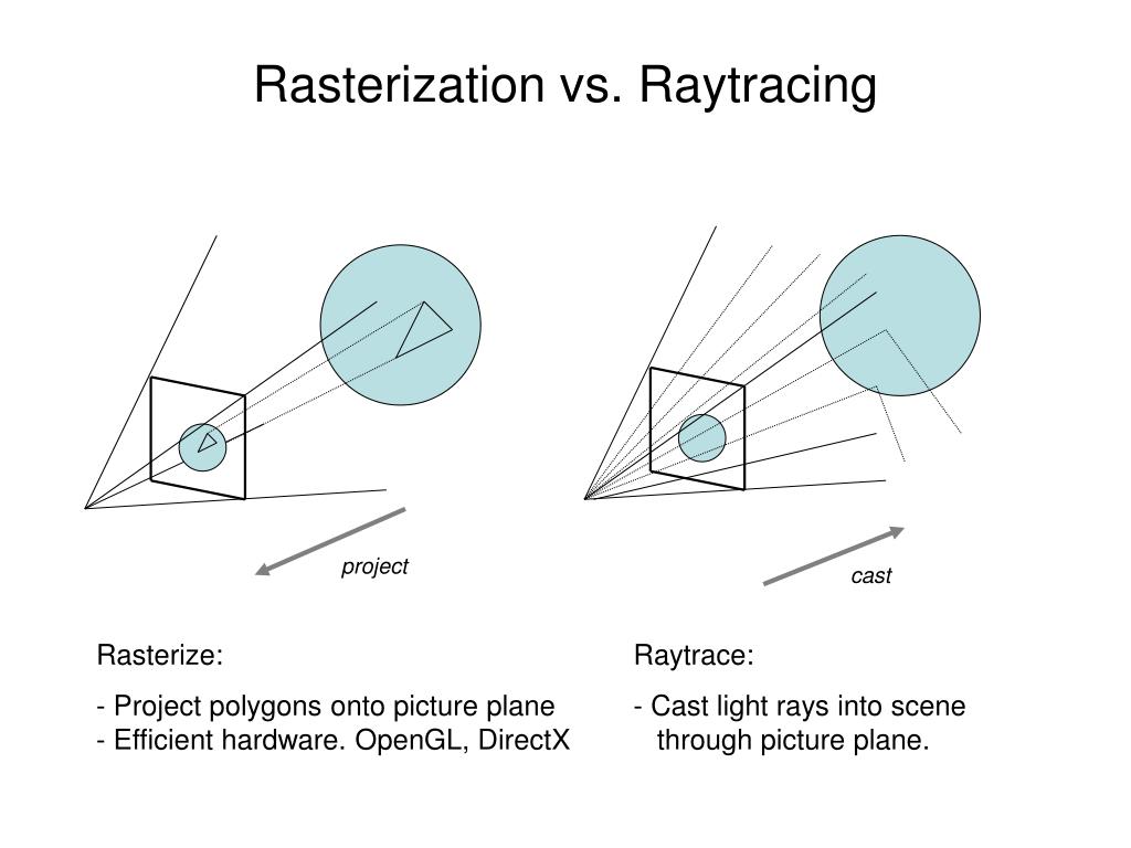
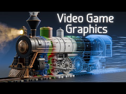
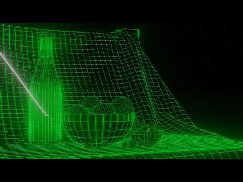
RASTERIZATION Rasterisation (or rasterization) is the task of taking the information described in a vector graphics format OR the vertices of triangles making 3D shapes and converting them into a raster image (a series of pixels, dots or lines, which, when displayed together, create the image which was represented via shapes), or in other words “rasterizing” vectors or 3D models onto a 2D plane for display on a computer screen.
For each triangle of a 3D shape, you project the corners of the triangle on the virtual screen with some math (projective geometry). Then you have the position of the 3 corners of the triangle on the pixel screen. Those 3 points have texture coordinates, so you know where in the texture are the 3 corners. The cost is proportional to the number of triangles, and is only a little bit affected by the screen resolution.
In computer graphics, a raster graphics orbitmap image is a dot matrix data structure that represents a generally rectangular grid of pixels (points of color), viewable via a monitor, paper, or other display medium.
With rasterization, objects on the screen are created from a mesh of virtual triangles, or polygons, that create 3D models of objects. A lot of information is associated with each vertex, including its position in space, as well as information about color, texture and its “normal,” which is used to determine the way the surface of an object is facing.
Computers then convert the triangles of the 3D models into pixels, or dots, on a 2D screen. Each pixel can be assigned an initial color value from the data stored in the triangle vertices.
Further pixel processing or “shading,” including changing pixel color based on how lights in the scene hit the pixel, and applying one or more textures to the pixel, combine to generate the final color applied to a pixel.
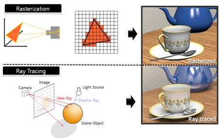
The main advantage of rasterization is its speed. However, rasterization is simply the process of computing the mapping from scene geometry to pixels and does not prescribe a particular way to compute the color of those pixels. So it cannot take shading, especially the physical light, into account and it cannot promise to get a photorealistic output. That’s a big limitation of rasterization.
There are also multiple problems:
If you have two triangles one is behind the other, you will draw twice all the pixels. you only keep the pixel from the triangle that is closer to you (Z-buffer), but you still do the work twice.
The borders of your triangles are jagged as it is hard to know if a pixel is in the triangle or out. You can do some smoothing on those, that is anti-aliasing.
You have to handle every triangles (including the ones behind you) and then see that they do not touch the screen at all. (we have techniques to mitigate this where we only look at triangles that are in the field of view)
Transparency is hard to handle (you can’t just do an average of the color of overlapping transparent triangles, you have to do it in the right order)
RAY CASTING It is almost the exact reverse of rasterization: you start from the virtual screen instead of the vector or 3D shapes, and you project a ray, starting from each pixel of the screen, until it intersect with a triangle.
The cost is directly correlated to the number of pixels in the screen and you need a really cheap way of finding the first triangle that intersect a ray. In the end, it is more expensive than rasterization but it will, by design, ignore the triangles that are out of the field of view.
You can use it to continue after the first triangle it hit, to take a little bit of the color of the next one, etc… This is useful to handle the border of the triangle cleanly (less jagged) and to handle transparency correctly.
RAYTRACING
Same idea as ray casting except once you hit a triangle you reflect on it and go into a different direction. The number of reflection you allow is the “depth” of your ray tracing. The color of the pixel can be calculated, based off the light source and all the polygons it had to reflect off of to get to that screen pixel.
The easiest way to think of ray tracing is to look around you, right now. The objects you’re seeing are illuminated by beams of light. Now turn that around and follow the path of those beams backwards from your eye to the objects that light interacts with. That’s ray tracing.
Ray tracing is eye-oriented process that needs walking through each pixel looking for what object should be shown there, which is also can be described as a technique that follows a beam of light (in pixels) from a set point and simulates how it reacts when it encounters objects.
Compared with rasterization, ray tracing is hard to be implemented in real time, since even one ray can be traced and processed without much trouble, but after one ray bounces off an object, it can turn into 10 rays, and those 10 can turn into 100, 1000…The increase is exponential, and the the calculation for all these rays will be time consuming.
Historically, computer hardware hasn’t been fast enough to use these techniques in real time, such as in video games. Moviemakers can take as long as they like to render a single frame, so they do it offline in render farms. Video games have only a fraction of a second. As a result, most real-time graphics rely on the another technique called rasterization.
PATH TRACING Path tracing can be used to solve more complex lighting situations. Path tracing is a type of ray tracing. When using path tracing for rendering, the rays only produce a single ray per bounce. The rays do not follow a defined line per bounce(to a light, for example), but rather shoot off in a random direction. The path tracing algorithm then takes a random sampling of all of the rays to create the final image. This results in sampling a variety of different types of lighting.
When a ray hits a surface it doesn’t trace a path to every light source, instead it bounces the ray off the surface and keeps bouncing it until it hits a light source or exhausts some bounce limit. It then calculates the amount of light transferred all the way to the pixel, including any color information gathered from surfaces along the way. It then averages out the values calculated from all the paths that were traced into the scene to get the final pixel color value.
It requires a ton of computing power and if you don’t send out enough rays per pixel or don’t trace the paths far enough into the scene then you end up with a very spotty image as many pixels fail to find any light sources from their rays. So when you increase the the samples per pixel, you can see the image quality becomes better and better.
Ray tracing tends to be more efficient than path tracing. Basically, the render time of a ray tracer depends on the number of polygons in the scene. The more polygons you have, the longer it will take. Meanwhile, the rendering time of a path tracer can be indifferent to the number of polygons, but it is related to light situation: If you add a light, transparency, translucence, or other shader effects, the path tracer will slow down considerably.
DISCLAIMER – Links and images on this website may be protected by the respective owners’ copyright. All data submitted by users through this site shall be treated as freely available to share.


