Disco Diffusion (DD) is a Google Colab Notebook which leverages an AI Image generating technique called CLIP-Guided Diffusion to allow you to create compelling and beautiful images from just text inputs. Created by Somnai, augmented by Gandamu, and building on the work of RiversHaveWings, nshepperd, and many others.
Colour is an open-source Python package providing a comprehensive number of algorithms and datasets for colour science. It is freely available under the BSD-3-Clause terms.
A LUT (Lookup Table) is essentially the modifier between two images, the original image and the displayed image, based on a mathematical formula. Basically conversion matrices of different complexities. There are different types of LUTS – viewing, transform, calibration, 1D and 3D.
By stimulating specific cells in the retina, the participants claim to have witnessed a blue-green colour that scientists have called “olo”, but some experts have said the existence of a new colour is “open to argument”.
The findings, published in the journal Science Advances on Friday, have been described by the study’s co-author, Prof Ren Ng from the University of California, as “remarkable”.
(A) System inputs. (i) Retina map of 103 cone cells preclassified by spectral type (7). (ii) Target visual percept (here, a video of a child, see movie S1 at 1:04). (iii) Infrared cellular-scale imaging of the retina with 60-frames-per-second rolling shutter. Fixational eye movement is visible over the three frames shown.
(B) System outputs. (iv) Real-time per-cone target activation levels to reproduce the target percept, computed by: extracting eye motion from the input video relative to the retina map; identifying the spectral type of every cone in the field of view; computing the per-cone activation the target percept would have produced. (v) Intensities of visible-wavelength 488-nm laser microdoses at each cone required to achieve its target activation level.
(C) Infrared imaging and visible-wavelength stimulation are physically accomplished in a raster scan across the retinal region using AOSLO. By modulating the visible-wavelength beam’s intensity, the laser microdoses shown in (v) are delivered. Drawing adapted with permission [Harmening and Sincich (54)].
(D) Examples of target percepts with corresponding cone activations and laser microdoses, ranging from colored squares to complex imagery. Teal-striped regions represent the color “olo” of stimulating only M cones.
One problem with sRGB is that in a gradient between blue and white, it becomes a bit purple in the middle of the transition. That’s because sRGB really isn’t created to mimic how the eye sees colors; rather, it is based on how CRT monitors work. That means it works with certain frequencies of red, green, and blue, and also the non-linear coding called gamma. It’s a miracle it works as well as it does, but it’s not connected to color perception. When using those tools, you sometimes get surprising results, like purple in the gradient.
There were also attempts to create simple models matching human perception based on XYZ, but as it turned out, it’s not possible to model all color vision that way. Perception of color is incredibly complex and depends, among other things, on whether it is dark or light in the room and the background color it is against. When you look at a photograph, it also depends on what you think the color of the light source is. The dress is a typical example of color vision being very context-dependent. It is almost impossible to model this perfectly.
I based Oklab on two other color spaces, CIECAM16 and IPT. I used the lightness and saturation prediction from CIECAM16, which is a color appearance model, as a target. I actually wanted to use the datasets used to create CIECAM16, but I couldn’t find them.
IPT was designed to have better hue uniformity. In experiments, they asked people to match light and dark colors, saturated and unsaturated colors, which resulted in a dataset for which colors, subjectively, have the same hue. IPT has a few other issues but is the basis for hue in Oklab.
In the Munsell color system, colors are described with three parameters, designed to match the perceived appearance of colors: Hue, Chroma and Value. The parameters are designed to be independent and each have a uniform scale. This results in a color solid with an irregular shape. The parameters are designed to be independent and each have a uniform scale. This results in a color solid with an irregular shape. Modern color spaces and models, such as CIELAB, Cam16 and Björn Ottosson own Oklab, are very similar in their construction.
By far the most used color spaces today for color picking are HSL and HSV, two representations introduced in the classic 1978 paper “Color Spaces for Computer Graphics”. HSL and HSV designed to roughly correlate with perceptual color properties while being very simple and cheap to compute.
Today HSL and HSV are most commonly used together with the sRGB color space.
One of the main advantages of HSL and HSV over the different Lab color spaces is that they map the sRGB gamut to a cylinder. This makes them easy to use since all parameters can be changed independently, without the risk of creating colors outside of the target gamut.
The main drawback on the other hand is that their properties don’t match human perception particularly well.
Reconciling these conflicting goals perfectly isn’t possible, but given that HSV and HSL don’t use anything derived from experiments relating to human perception, creating something that makes a better tradeoff does not seem unreasonable.
With this new lightness estimate, we are ready to look into the construction of Okhsv and Okhsl.
A number of problems in computer vision and related fields would be mitigated if camera spectral sensitivities were known. As consumer cameras are not designed for high-precision visual tasks, manufacturers do not disclose spectral sensitivities. Their estimation requires a costly optical setup, which triggered researchers to come up with numerous indirect methods that aim to lower cost and complexity by using color targets. However, the use of color targets gives rise to new complications that make the estimation more difficult, and consequently, there currently exists no simple, low-cost, robust go-to method for spectral sensitivity estimation that non-specialized research labs can adopt. Furthermore, even if not limited by hardware or cost, researchers frequently work with imagery from multiple cameras that they do not have in their possession.
To provide a practical solution to this problem, we propose a framework for spectral sensitivity estimation that not only does not require any hardware (including a color target), but also does not require physical access to the camera itself. Similar to other work, we formulate an optimization problem that minimizes a two-term objective function: a camera-specific term from a system of equations, and a universal term that bounds the solution space.
Different than other work, we utilize publicly available high-quality calibration data to construct both terms. We use the colorimetric mapping matrices provided by the Adobe DNG Converter to formulate the camera-specific system of equations, and constrain the solutions using an autoencoder trained on a database of ground-truth curves. On average, we achieve reconstruction errors as low as those that can arise due to manufacturing imperfections between two copies of the same camera. We provide predicted sensitivities for more than 1,000 cameras that the Adobe DNG Converter currently supports, and discuss which tasks can become trivial when camera responses are available.
Björn Ottosson proposed OKlch in 2020 to create a color space that can closely mimic how color is perceived by the human eye, predicting perceived lightness, chroma, and hue.
The OK in OKLCH stands for Optimal Color.
L: Lightness (the perceived brightness of the color)
C: Chroma (the intensity or saturation of the color)
H: Hue (the actual color, such as red, blue, green, etc.)
Basically, gamma is the relationship between the brightness of a pixel as it appears on the screen, and the numerical value of that pixel. Generally Gamma is just about defining relationships.
Three main types: – Image Gamma encoded in images – Display Gammas encoded in hardware and/or viewing time – System or Viewing Gamma which is the net effect of all gammas when you look back at a final image. In theory this should flatten back to 1.0 gamma.
About 576 megapixels for the entire field of view.
Consider a view in front of you that is 90 degrees by 90 degrees, like looking through an open window at a scene. The number of pixels would be:
90 degrees * 60 arc-minutes/degree * 1/0.3 * 90 * 60 * 1/0.3 = 324,000,000 pixels (324 megapixels).
At any one moment, you actually do not perceive that many pixels, but your eye moves around the scene to see all the detail you want. But the human eye really sees a larger field of view, close to 180 degrees. Let’s be conservative and use 120 degrees for the field of view. Then we would see:
“a simple yet effective technique to estimate lighting in a single input image. Current techniques rely heavily on HDR panorama datasets to train neural networks to regress an input with limited field-of-view to a full environment map. However, these approaches often struggle with real-world, uncontrolled settings due to the limited diversity and size of their datasets. To address this problem, we leverage diffusion models trained on billions of standard images to render a chrome ball into the input image. Despite its simplicity, this task remains challenging: the diffusion models often insert incorrect or inconsistent objects and cannot readily generate images in HDR format. Our research uncovers a surprising relationship between the appearance of chrome balls and the initial diffusion noise map, which we utilize to consistently generate high-quality chrome balls. We further fine-tune an LDR difusion model (Stable Diffusion XL) with LoRA, enabling it to perform exposure bracketing for HDR light estimation. Our method produces convincing light estimates across diverse settings and demonstrates superior generalization to in-the-wild scenarios.”
“Unless you have all the relevant spectral measurements, a colour rendition chart should not be used to perform colour-correction of camera imagery but only for white balancing and relative exposure adjustments.”
“Using a colour rendition chart for colour-correction might dramatically increase error if the scene light source spectrum is different from the illuminant used to compute the colour rendition chart’s reference values.”
“other factors make using a colour rendition chart unsuitable for camera calibration:
– Uncontrolled geometry of the colour rendition chart with the incident illumination and the camera.
– Unknown sample reflectances and ageing as the colour of the samples vary with time.
– Low samples count.
– Camera noise and flare.
– Etc…
“Those issues are well understood in the VFX industry, and when receiving plates, we almost exclusively use colour rendition charts to white balance and perform relative exposure adjustments, i.e. plate neutralisation.”
An exposure stop is a unit measurement of Exposure as such it provides a universal linear scale to measure the increase and decrease in light, exposed to the image sensor, due to changes in shutter speed, iso and f-stop.
+-1 stop is a doubling or halving of the amount of light let in when taking a photo
1 EV (exposure value) is just another way to say one stop of exposure change.
Same applies to shutter speed, iso and aperture.
Doubling or halving your shutter speed produces an increase or decrease of 1 stop of exposure.
Doubling or halving your iso speed produces an increase or decrease of 1 stop of exposure.
The dynamic range is a ratio between the maximum and minimum values of a physical measurement. Its definition depends on what the dynamic range refers to.
For a scene: Dynamic range is the ratio between the brightest and darkest parts of the scene.
For a camera: Dynamic range is the ratio of saturation to noise. More specifically, the ratio of the intensity that just saturates the camera to the intensity that just lifts the camera response one standard deviation above camera noise.
For a display: Dynamic range is the ratio between the maximum and minimum intensities emitted from the screen.
The Dynamic Range of real-world scenes can be quite high — ratios of 100,000:1 are common in the natural world. An HDR (High Dynamic Range) image stores pixel values that span the whole tonal range of real-world scenes. Therefore, an HDR image is encoded in a format that allows the largest range of values, e.g. floating-point values stored with 32 bits per color channel. Another characteristics of an HDR image is that it stores linear values. This means that the value of a pixel from an HDR image is proportional to the amount of light measured by the camera.
For TVs HDR is great, but it’s not the only new TV feature worth discussing.
DISCLAIMER – Links and images on this website may be protected by the respective owners’ copyright. All data submitted by users through this site shall be treated as freely available to share.


